All published articles of this journal are available on ScienceDirect.

Team Chemistry and COVID in European Football
Abstract
Objective:
This research investigates the influence of team chemistry and COVID on football matches.
Methods:
This is done by estimating the effect of both chemistryand COVID on match results and analysing the performance of prediction models where both effects are included and threshold intervals are usedfor classification. Four different chemistry measures are introduced and all are evaluated.
Results:
Chemistry has the expected positive effect on performance only for the top teams in the estimations where interaction effects are included for two different chemistry measures. COVID has the expected mitigating effect on home advantage.
The inclusion of both effects in prediction models does not increase prediction accuracy consistently, although for various symmetric threshold intervals the prediction models with chemistry and COVID included outperforming the baseline models.
Conclusion:
Chemistry can have a positive influence on the perfomrance of a team and empty stadiums due to COVID mitigate the effect of home advantage. Including COVID and chemistry measures based on region in predictions is highly recommended.
1. INTRODUCTION
Football is the most popular sport in the world, and predictions are made daily for football matches. Money can be earned with smart betting and eternal glory can be achieved by beating your friends and family with Scorito. But how is a good prediction made? One of the main influences on the strength of a team which is often forgotten is chemistry. Teams that do not have the best players can still beat the top teams. Take, for example, Leicester, which won the Premier League in 2016 or Villareal, which made the Champions League semi-final this season. As head coach of The Netherlands (10th on the FIFA world ranking) Louis van Gaal said after his team destroyed Belgium, the number two on the FIFA world ranking, with 1-4, 'this is a victory of the collective'. This often happens because the players in these teams are so well attuned to each other that the team's overall quality outperforms the seemingly superior individual quality of the opposition's players. This so-called chemistry is something from which a lot can be learned.
During the recent COVID pandemic, essential things have changed in football. The stadiums were empty for almost an entire season, which enormously impactedhe matches played in this period [1]. Investigating the impact of COVID on football matches is vital to get a clear picture of what determines the outcome of a football match.
This paper will investigate what influence chemistry has on the outcome of football matches. Furthermore, the impact of COVID and the accuracy of predicting football matches is of great concern.
Chemistry has not been used in football predictions before. Since chemistry has a major influence on the outcome of a football match [2], it should not be omitted in making predictions.
If chemistry can be captured in a single number, this would create a new variable that can predict surprise outcomes and decrease the randomness in predictions. Finding this chemistry measure would open a new world in the area of team sport and particular, football predictions.
The research will be performed with extensive data consisting of four datasets combined into one extensive panel dataset [3]. The data consists of over 44 thousand matches played in 10 years in which more than 22 thousand players made an appearance for 400 different clubs. The data are combined into one big dataset that contains all the necessary information. A more extended explanation of the data is given in the Data section.
Various models will be used to measure the effect of chemistry on the outcomes of football matches and make predictions. The model that will be used for the prediction of football matches and the estimation of impacts of chemistry variables and other parameters is the Two-Way Fixed Effects model. This model is designed to capture both time and club-specific effects in the panel data structure.
The biggest challenge is to find an elegant way to measure chemistry. Four different methods will be used to measure the chemistry based on nationality or region players come from. The two different ways to get the eventual normalised number for chemistry are to use the Social Connectedness Index [4] and the largest eigenvalue method.
The Two-Way Fixed Effects model is used since the data are panel data and panel regression can capture time and club-specific effects that would otherwise be missed. Furthermore, the methods to measure chemistry are brand new since including this has never been done before. Nationality and region are used since communication is vital in football and coming from the same country or region will help communicate easier and thus increase chemistry. The methods used to measure the chemistry are carefully thought out and will be explained in more detail in the Methodology section.
One of the main findings is that chemistry negatively affects performance in most cases, which does not interfere with expectations. After fine-tuning the model, chemistry has a positive effect on performance for the top teams, although the effect on performance for less-skilled teams is still negative.
Another important finding is that COVID is estimated to have a mitigating effect on home advantage as the estimates of COVID in all estimations are negative and significant in most of them. This means that leaving fans out of the stadium will reduce a home team's advantage of playing in its own stadium. This is in accordance with the findings of Tilp and Thaller [5].
Adding both chemistry and COVID to the prediction model leads to an occasional outperformance of the baseline models and certainly not a structural outperformance by the baseline models. Therefore, the inclusion of chemistry and COVID in football prediction models is highly recommended in further research.
The paper contains a Literature Review section followed by a detailed description of the Data. The Methodology is of interest in the next section, followed by the Results. Lastly, the results will be discussed and a conclusion will be given in the Discussion section.
2. LITERATURE REVIEW
Football is the most popular sport in the world [6]. Various studies have been done regarding football ranging from match analysis [7] to risk factor analysis for injuries [8]. Analysis of specific factors that influence a game’s outcome, such as the referee-bias [9] is also one of the main fields in football research. Predicting football matches is also a subject of interest in football literature. With the premature ending of the Dutch and French competition, a prediction of the final standings is performed by Gorgi, Koopman, and Lit [10]. Studying the influence of a single feature in sports, especially football, is difficult due to the dynamic nature of the game and the countless factors that can influence the final result [11]. A few factors that influence the final result are the strength of the home and the away team, the weather, the form both teams are in, the possible injuries of players and go on. A, in research, often forgotten or omitted factor of influence is team chemistry and chemistry between players. Take, for example, the chemistry between Spanish midfield wizards Xavi and Iniesta [12] that took FC Barcelona to incredible triumphs. Without their chemistry with each other and the rest of the team, Barça would not have been able to achieve their success.
This chemistry is, however, hard to measure since there are many factors that influence team chemistry [13]. Interaction among players is one of the most important influences on chemistry. This can be divided into many different components ranging from professional understanding to players’ emotional intelligence. In-group favouritism [14] and, in particular, ethnicity can play a significant role in this interaction among players. Since the data contains information on players’ origins and because of the expected influence of in-group favouritism, the chemistry measure in this research will be based on nationality.
A method to measure chemistry or connectedness within a group is proposed by [4], which measures the connectedness between and within countries or counties through Facebook friendships. The method they introduce is, however, widely applicable. The Social Connectedness Index, or SCI, as Bailey et al. [4] call it, uses a simple formula that can be used in whatever desired field as long as there is a connection matrix. This measure is, for example, used to predict and explain the spread of diseases such as COVID [15] during times of pandemic.
In football prediction literature, the model that is used most often is a bivariate Poisson model first introduced by Maher [16] and later fine-tuned by Dixon & Coles [17] and Gorgi et al. [10]. These models are based on historical results and these are used to find parameters for the attacking and defensive strength and home advantage [18] of the researched teams. Those parameters will absorb all other factors that possibly influence the outcome of a match.
Including these absorbed and omitted variables in the model can provide a clearer picture of what is happening in football matches.
Including these effects in the Bivariate Poisson model will lead to an enormous number of parameters that must be estimated. Furthermore, many factors that differ per match are not taken into account. To account for the unobserved heterogeneity of the factors that cannot be considered, a Two-Way Fixed Effects Regression Model [19] will be used in this research. A Bivariate Poisson model with the addition of other factors is likely to cause identification issues. This means a two-way fixed effects regression model is preferred over an extended Bivariate Poisson model. The first hypothesis is that chemistry has a positive effect on performance for both the home and away team. The second hypothesis is that COVID has a mitigating effect on home advantage. The third hypothesis is that including chemistry improves predictions and the last hypothesis is that including COVID improves predictions.
2.1. Data
The data used in this research is very extensive. The dataset is retrieved from Transfermarkt.com and put together by Cereijo [3]. The data consists of four different datasets that are linked by codes. There is a dataset for players, clubs, games and appearances. Those are put together via player ids, game ids and club ids so that the desired format is reached eventually. A description of how this is done precisely can be found in the Appendix. The dataset that is eventually used needs some explanation. The dataset consists of 44.666 games from July 9th, 2012 (Metalurg Donetsk - Shakhtar Donetsk) until April 11th, 2022 (Antalyaspor - Hatayspor and Bologna - Sampdoria). Four hundred clubs play these games in 35 different domestic competitions in 14 different countries and four different European competitions. In these games, many players participated. The appearances of 17851 players from 171 countries are recorded in the dataset. This means that the number of observations is substantial and accurate results can be achieved. In the following subsections, the data will be further explained.
2.2. Variables
The cleaned dataset contains numerous variables that will be listed and explained in this paragraph.
2.2.1. Dependent Variable
- Goal Difference: the number of goals scored by the home team minus the number of goals scored by the away team. For example, the match between FC Barcelona and Real Madrid played on October 28th, 2018, ended 5-1. The number of goals scored by the home team, FC Barcelona, is five and the number of goals scored by the away team, Real Madrid, is one. The variable Goal Difference will take the value 5 − 1 = 4. In case of a draw, the variable Goal Difference will thus be 0 as the number of home and away goals are the same. In case of a win by the home team, as explained in the example, the value of the variable Goal Difference will be positive. Finally, in case of a win by the away team, the value of the variable Goal Difference will be negative.
2.2.2. Explanatory Variables
- Home Chemistry: the chemistry of the home team. The chemistry variables are the variables of interest in this research. The calculation of this variable will be explained in more detail in the Statistics section.
- Away Chemistry: the chemistry of the away team. The chemistry variables are the variables of interest in this research. The calculation of this variable will be explained in more detail in the Statistics section.
- COVID/No Attendance: a dummy variable that indicates if the game is played in COVID times or without attendance. The dummy is equal to one if a game is played in without attendance and zero otherwise.
- Home Height: the mean height of the home team in centimeters.
- Away Height: the mean height of the away team in centimeters.
- Home Age: the mean age of the home team in years.
- Away Age: the mean age of the away team in years.
- Home Position: the ranking of the home team at the time of the match. The lower the value the higher the team is ranked.
- Away Position: the ranking of the away team at the time of the match. The lower the value the higher the team is ranked.
- Dummies: to control for country-specific effects dummies will be added to the dataset. A dummy is one if a game is played in a domestic competition (league, cup, super cup) in a specific country or if a game is played in a European competition. The dummies are Europe, Spain, Portugal, Russia, Italy, Germany, Netherlands, England, Ukraine, Scotland, France, Greece, Belgium, Denmark, Turkey. These are the fourteen countries in which the games are played and Europe for the games that are played in a European competition.
2.3. Statistics
In this section, (descriptive) statistics of all variables can be found. First, the calculation of the chemistry variables will be discussed. After that, descriptive statistics of the chemistry and other variables will be shown and discussed.
2.4. Chemistry
The most important variables in this research are the chemistry variables. The question remains about how to measure this chemistry variable. Four methods are proposed to measure this abstract variable. As in-group favouritism [14] and, in particular, ethnicity possibly play an important role, this ethnic component will be used as a measure for chemistry. The ethnic component of the measure is divided into strict and loose measures. The strict measure is based on the nationality of the players and the loose measure is based on the part of the world (in this research, the world is divided into eight parts) the players come from. The proposed methods start with all the players that play for a specific team in a specific match (both starters and substitutes). Take, for example, Ajax in the heroic comeback in the Champions League in 2019. The players that played for Ajax in that match are listed in Table 1. From this information a n × n connection matrix A is constructed. The entries in the matrix are either 0 or 1. An entry αij will take the value 1 if player i and player j have the same nationality (or region). The diagonal will thus be filled with ones as, there, a player is compared to itself. Two methods to calculate the chemistry of a team in a match will be proposed.
2.5. Social Connectedness Index (SCI)
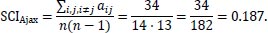
The matrix to calculate the chemistry from the nationalities in Table 1 can be found in Table 2. From this matrix, the number for chemistry will be calculated. The first method to calculate the chemistry from this matrix is the Social Connectedness Index or SCI [4].The Social Connectedness Index counts the number of connections in this matrix the ones, and divides it by the total possible number of connections. This division is done to normalise the measure. The minimal value is zero and the maximum value is one. As a player always will have a connection with itself, the diagonal ones will be omitted in the calculation. In formula form, the Social Connectedness Index looks as follows
 |
In the example, a connection is formed when two players have the same nationality. The number of ones in the example is 48. After subtracting the diagonal ones, 34 connections remain. As n = 14, the SCI for Ajax in this particular match can be calculated.
 |
A connection can also be formed if players come from the same region. Using the SCI to calculate the chemistry thus delivers two different chemistry measures. A possible direction in future research can be to combine the region and nationality measures and weight, for example, the region connections with a factor of 0.5.
2.6. Largest Eigenvalue (LE)
The matrix to calculate the chemistry from the regions in Table 1 is shown in Table 3. The second method to calculate the chemistry from these matrices is the largest eigenvalue method. The eigenvalues are calculated with the equation
 |
with x a nonzero vector. The matrix will have n eigenvalues. In this case, the matrices are always symmetric and many rows are the same. The largest eigenvalue will be equal to the largest cluster of players from the same nationality or region. In the Ajax example, there are six Dutchmen, two Moroccans, two Danes, a Serbian, an Argentine, a Brazilian and a Cameroonian. The largest eigenvalue will thus be 6. In order to make the measure comparable over the whole sample with different n, the largest eigenvalue λ1 is divided by the number of players that played for a team in a certain match. The largest eigenvalue chemistry measure (LE) looks as follows
 |
From the Ajax example in Table 1, the region matrix in Table 3 is constructed. The biggest cluster in the region matrix is from European players. There are nine European players, three Africans and two South Americans. The largest eigenvalue from the region matrix will thus be equal to 9. The region chemistry based on the largest eigenvalue method for Ajax in this match is
 |
2.7. Descriptive Statistics
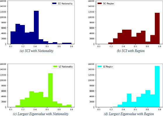
To illustrate the differences between the measures, the descriptive statistics in Table 4 and histograms of the different chemistry measures in Fig. (1) are shown below. As can be seen from Table 4 and Fig. (1a), the chemistry measure based on nationality and calculated with the SCI is the most conservative. This can be deducted from the relatively low mean (0.292) and from the histogram that shows almost all mass is below 0.5. The chemistry measure based on nationality and calculated with the largest eigenvalue method is more evenly spread out, as can be seen in Fig. (1c). There is, however, a peak around 0.65. This peak is caused by the occurrence of 8 players from the same country in a match where 13 different players played for a specific team. If this occurs, the chemistry measure calculated with the SCI will lie in the interval (0.442,0.571), explaining the peak around 0.45 in Fig. (1a). The use of the chemistry measure based on region shifts mass to one as there are a lot more connections due to the reduction of possible regions from 171 countries to 8 parts of the world. This shift is both visible in (Table 4 and Fig. 1b and 1d) as the means are above 2/3 and mass is shifted to the right with peaks in the rightmost interval that ends at one. Once again, the SCI is somewhat more conservative than the largest eigenvalue measure as the mean and minimum are somewhat lower (Table 4) in comparison with the largest eigenvalue measure. This is due to the nature of the measure as in the example, the largest cluster of 8 players from the same region out of 13 that participated for that particular team in that particular match will lead to a chemistry measure of
 |
In contrast, the chemistry measure calculated with the SCI in this example cannot exceed 0.571.
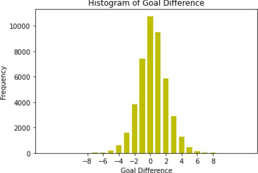
From Fig. (2) can be seen that the Goal Difference is centered around zero with 10753 draws which are 24.1% of the data. The number of matches with a negative goal difference is 13730. This means 13730 (30.7%) matches are won by the away team. The remaining 20183 (45.2%) matches are won by the home team. This domination of wins by the home team can be explained by a phenomenon called home advantage [18]; [20]. This home advantage will not be taken into consideration as the data do not provide the necessary detailed information that is needed. It is likely to be captured by the constant term as it is a sort of measure for home advantage already (Table 5). The sign of the constant term will, however, not give any information since most control variables have a positive minimum and maximum value that will be added to the constant term. As can be seen from Table 6, the variables Home Height and Away Height, Home Age and Away Age and Home Position and Away Position all are quite similar in terms of possible home and away the difference. The means of the dummy variables show what part of the sample is classified in that dummy group. This means 13.66% of all matches are played without attendance during COVID and 7.084% of all matches are played in a Dutch competition. In the case of the Netherlands, a match can be played in the Dutch League (Eredivisie), the Dutch Cup (KNVB Beker) or the Dutch Super Cup (Johan Cruijff Schaal).
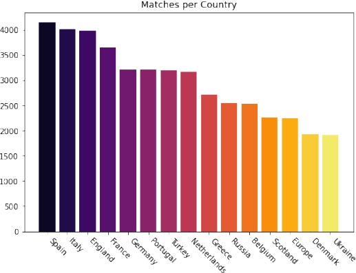
From Fig. (3) can be seen that most matches are played in a Spanish competition (4141), followed by Italian and English competitions. The least matches are played in Ukrainian (1916) and Danish (1918) Competitions. The matches are evenly spread over the countries, with parts that range from 4.29% to 9.27%. This means the number of matches in the different countries is big enough to detect differences between countries. The variable that will eventually be estimated is the goal difference. The variables of interest are the chemistry variables. To give some more insight into the behaviour of those variables, some interesting correlations will be shown in Table 7. As can be seen from this table, the correlation of height and age with goal difference is very close to zero, although the home and away parts are all opposite. The correlation of position with Goal Difference is quite large, with -0.3726 for Home Position and 0.3616 for Away Position. This is as expected, as the better a team, the bigger the goal difference. As a team is better when the value of position is lower, the sign of the correlation of Goal Difference and Home Position is negative and the sign of the correlation of Goal Difference and Away Position is positive.
| Players | i | Nationality | Region |
|---|---|---|---|
| Dani de Wit | 1 | Netherlands | Europe |
| Matthijs de Ligt | 2 | Netherlands | Europe |
| Lasse Schone | 3 | Denmark | Europe |
| Nicolas Tagliafico | 4 | Argentina | South America |
| Joel Veltman | 5 | Netherlands | Europe |
| Frenkie de Jong | 6 | Netherlands | Europe |
| Andre Onana | 7 | Cameroon | Africa |
| Donny van de Beek | 8 | Netherlands | Europe |
| Kasper Dolberg | 9 | Denmark | Europe |
| Daley Blind | 10 | Netherlands | Europe |
| Hakim Ziyech | 11 | Morocco | Africa |
| David Neres | 12 | Brazil | South America |
| Noussair Mazraoui | 13 | Morocco | Africa |
| Dusan Tadic | 14 | Serbia | Europe |
| i \ j | 1 | 2 | 3 | 4 | 5 | 6 | 7 | 8 | 9 | 10 | 11 | 12 | 13 | 14 |
|---|---|---|---|---|---|---|---|---|---|---|---|---|---|---|
| 1 | 1 | 1 | 0 | 0 | 1 | 1 | 0 | 1 | 0 | 1 | 0 | 0 | 0 | 0 |
| 2 | 1 | 1 | 0 | 0 | 1 | 1 | 0 | 1 | 0 | 1 | 0 | 0 | 0 | 0 |
| 3 | 0 | 0 | 1 | 0 | 0 | 0 | 0 | 0 | 1 | 0 | 0 | 0 | 0 | 0 |
| 4 | 0 | 0 | 0 | 1 | 0 | 0 | 0 | 0 | 0 | 0 | 0 | 0 | 0 | 0 |
| 5 | 1 | 1 | 0 | 0 | 1 | 1 | 0 | 1 | 0 | 1 | 0 | 0 | 0 | 0 |
| 6 | 1 | 1 | 0 | 0 | 1 | 1 | 0 | 1 | 0 | 1 | 0 | 0 | 0 | 0 |
| 7 | 0 | 0 | 0 | 0 | 0 | 0 | 1 | 0 | 0 | 0 | 0 | 0 | 0 | 0 |
| 8 | 1 | 1 | 0 | 0 | 1 | 1 | 0 | 1 | 0 | 1 | 0 | 0 | 0 | 0 |
| 9 | 0 | 0 | 1 | 0 | 0 | 0 | 0 | 0 | 1 | 0 | 0 | 0 | 0 | 0 |
| 10 | 1 | 1 | 0 | 0 | 1 | 1 | 0 | 1 | 0 | 1 | 0 | 0 | 0 | 0 |
| 11 | 0 | 0 | 0 | 0 | 0 | 0 | 0 | 0 | 0 | 0 | 1 | 0 | 1 | 0 |
| 12 | 0 | 0 | 0 | 0 | 0 | 0 | 0 | 0 | 0 | 0 | 0 | 1 | 0 | 0 |
| 13 | 0 | 0 | 0 | 0 | 0 | 0 | 0 | 0 | 0 | 0 | 1 | 0 | 1 | 0 |
| 14 | 0 | 0 | 0 | 0 | 0 | 0 | 0 | 0 | 0 | 0 | 0 | 0 | 0 | 1 |
| i \ j | 1 | 2 | 3 | 4 | 5 | 6 | 7 | 8 | 9 | 10 | 11 | 12 | 13 | 14 |
|---|---|---|---|---|---|---|---|---|---|---|---|---|---|---|
| 1 | 1 | 1 | 1 | 0 | 1 | 1 | 0 | 1 | 1 | 1 | 0 | 0 | 0 | 1 |
| 2 | 1 | 1 | 1 | 0 | 1 | 1 | 0 | 1 | 1 | 1 | 0 | 0 | 0 | 1 |
| 3 | 1 | 1 | 1 | 0 | 1 | 1 | 0 | 1 | 1 | 1 | 0 | 0 | 0 | 1 |
| 4 | 0 | 0 | 0 | 1 | 0 | 0 | 0 | 0 | 0 | 0 | 0 | 1 | 0 | 0 |
| 5 | 1 | 1 | 1 | 0 | 1 | 1 | 0 | 1 | 1 | 1 | 0 | 0 | 0 | 1 |
| 6 | 1 | 1 | 1 | 0 | 1 | 1 | 0 | 1 | 1 | 1 | 0 | 0 | 0 | 1 |
| 7 | 0 | 0 | 0 | 0 | 0 | 0 | 1 | 0 | 0 | 0 | 1 | 0 | 1 | 0 |
| 8 | 1 | 1 | 1 | 0 | 1 | 1 | 0 | 1 | 1 | 1 | 0 | 0 | 0 | 1 |
| 9 | 1 | 1 | 1 | 0 | 1 | 1 | 0 | 1 | 1 | 1 | 0 | 0 | 0 | 1 |
| 10 | 1 | 1 | 1 | 0 | 1 | 1 | 0 | 1 | 1 | 1 | 0 | 0 | 0 | 1 |
| 11 | 0 | 0 | 0 | 0 | 0 | 0 | 1 | 0 | 0 | 0 | 1 | 0 | 1 | 0 |
| 12 | 0 | 0 | 0 | 1 | 0 | 0 | 0 | 0 | 0 | 0 | 0 | 1 | 0 | 0 |
| 13 | 0 | 0 | 0 | 0 | 0 | 0 | 1 | 0 | 0 | 0 | 1 | 0 | 1 | 0 |
| 14 | 1 | 1 | 1 | 0 | 1 | 1 | 0 | 1 | 1 | 1 | 0 | 0 | 0 | 1 |
| Chemistry Measure | Mean | Standard Deviation | Min | Max |
|---|---|---|---|---|
| SCI | 0.292 | 0.178 | 0 | 1 |
| LE | 0.506 | 0.172 | 0.0714 | 1 |
| SCI Region | 0.669 | 0.249 | 0.128 | 1 |
| LE Region | 0.776 | 0.192 | 0.214 | 1 |
| Chemistry Measure | Correlation with Goal Difference |
|---|---|
| Home SCI | -0.06253 |
| Away SCI | 0.05662 |
| Home LE | -0.06674 |
| Away LE | 0.06414 |
| Home SCI Region | -0.02246 |
| Away SCI Region | 0.01687 |
| Home LE Region | -0.02185 |
| Away LE Region | 0.01374 |
3. METHODOLOGY
In the following section, the model and different chemistry measures will be elaborated on. In the last section, the differences between the different chemistry measures will be treated with descriptive statistics.
3.1. Model
The baseline model that will be used is the Two-Way Fixed Effects model. This is a panel regression model that controls for time-fixed effects and team-specific effects. The model is
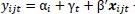 |
with yijt the goal difference between home team i and away team j played in time period t. Time period t is chosen as a quarter, so t = 0, ..., 39 as the matches are played over ten years or forty quarters time. The match-specific variables xijt are the variables of interest, Home Chemistry and Away Chemistry, control variables such as Home Position and Away Age that differ per match as mentioned in the Explanatory Variables section and interaction effects between the variables of interest and the control variables. To check robustness, country-specific dummies will be added. In other words, these dummies check for differences between matches played in different countries. The added dummies are as mentioned in the Explanatory Variables section, with one left out as the baseline country. The England dummy will be used as the baseline country to which the other dummies will be compared. The model to check for these country-specific effects looks as follows
 |
with Dijt a vector where the entry corresponding to the country the competition is from is equal to one and the rest of the entries equal to zero. These dummies are not redundant as a team can play both in domestic competition and Europe, so there is no one-to-one correspondence between a team and the country dummy. The models, as mentioned above, are, however, implicit. Since for every i and every t, a fixed effect is present, estimating this model will give identification issues due to the large number of parameters that must be estimated. To get rid of those fixed effects ”double-demeaning” is used [21].
Define the team-specific averages over time as
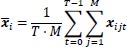 |
and
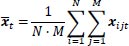 |
the cross-sectional average for each time-period t. The total average is
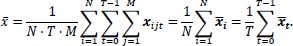 |
Define
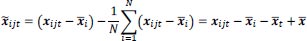 |
and similarly
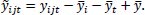 |
In the equations above t ranges from 0 to 39 but does not necessarily take all those values given a specific t,T therefore, ranges from 1 up to 40. For i and j hold similar reasoning, i ranges from 1 to 400 but does not need to take all values for a specific t. N can therefore range from 1 to 400. The range of j, which differentiates between matches that team i plays in time period t, is from 1 to 13 and can take any value in between. M can therefore range from 1 to 13. The estimates are eventually found by regression of y~ijt on x~ijt. The equation to find ^β is
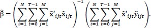 |
The two-way fixed effect model can be expressed as a Least Squares Dummy Variable (LSDV) estimator that in the formula is
 |
where d1,i and d2,t are the dummy variables for the team-specific and time effects [22].
For the variance-covariance estimator, a clustered variance-covariance estimator is used. This is done to make sure the differences between the time and team clusters are taken into account in calculating the variance-covariance estimator. In formula
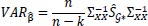 |
where
 |
and
 |
where
 |
and ijt Ɛ Gg indicates that the observation belongs to group g. Groups g are the different clusters. In the case of two-way clustering used in this estimation, there is a cluster for each different i, t and it. For example, there are separate clusters for matches in which AZ Alkmaar is the home team, for matches played in the 29th quarter of the dataset (t = 29) and for matches played in the 29th quarter of the dataset (t = 29) with AZ Alkmaar as the home team.
3.2. Predictions
Predicting matches is the most exciting thing that can be done with all the information gathered from the estimations. These predictions will be made with the model that is estimated and the information available for a new match. A prediction can thus be made shortly before a match since then, the line-ups are known and the corresponding chemistry measures can be calculated. Moreover, the average height of both teams and the average age of both teams also need to be calculated to make the predictions as accurate as possible.
The forecasts that will be made are, however, not likely to be integers. This means the forecasts will be made on the match’s so-called ’toto’ outcome. The ’toto’ outcome means if the home or away team wins the match or if the match ends in a draw. This is less specific than the goal difference, as the goal difference also measures the magnitude of a win. The second part of the predictions is to determine threshold values for the classification in either of the three classes [20]. These threshold values will form a symmetric or asymmetric interval around zero. If the predicted goal difference is in the interval, a draw will be forecast for that match. If the predicted goal difference is outside the interval, either a home win (positive sign) or away win (negative sign) is predicted depending on the sign of the predicted goal difference.
The threshold interval will be determined by k-fold cross-validation [23]. This method splits the dataset into k parts and takes one of those k parts as test set and the remaining k − 1 parts as training set. The training set is used to estimate the model with which the test set will be predicted. Then the predicted outcomes of the test set will be compared to the actual outcomes of the test set. This will be done k-times with all k different parts of the data once used as the test set. Usually, 5 or 10-fold cross-validation is used and in this research, 5-fold cross-validation will be used. A confusion matrix will be created to determine how good the predictions are. This confusion matrix is shown in Table 8.

| Variable | Mean | Standard Deviation | Min | Max |
|---|---|---|---|---|
| Goal Difference | 0.3313 | 1.832 | -13 | 10 |
| Home Height (in cm) | 181.2 | 2.318 | 174.5 | 189.1 |
| Away Height (in cm) | 182.1 | 1.560 | 174.4 | 189.6 |
| Home Age (in years) | 26.88 | 1.547 | 18.56 | 37.18 |
| Away Age (in years) | 26.22 | 1.636 | 18.72 | 34.59 |
| Home Position | 9.010 | 5.367 | 1 | 21 |
| Away Position | 9.198 | 5.390 | 1 | 21 |
| COVID/No Attendance* | 0.1366 | 0.3434 | 0 | 1 |
| Ukraine* | 0.04290 | 0.2026 | 0 | 1 |
| Denmark* | 0.04294 | 0.2027 | 0 | 1 |
| Russia* | 0.05693 | 0.2317 | 0 | 1 |
| Europe* | 0.05024 | 0.2184 | 0 | 1 |
| Turkey* | 0.07137 | 0.2574 | 0 | 1 |
| Belgium* | 0.05671 | 0.2313 | 0 | 1 |
| Scotland* | 0.05049 | 0.2189 | 0 | 1 |
| France* | 0.08147 | 0.2736 | 0 | 1 |
| Portugal* | 0.07178 | 0.2581 | 0 | 1 |
| Greece* | 0.06078 | 0.2389 | 0 | 1 |
| Netherlands* | 0.07084 | 0.2566 | 0 | 1 |
| Italy* | 0.08980 | 0.2859 | 0 | 1 |
| Germany* | 0.07191 | 0.2583 | 0 | 1 |
| England* | 0.08913 | 0.2849 | 0 | 1 |
| Spain* | 0.09271 | 0.2900 | 0 | 1 |
| Variable | Correlation with Goal Difference |
|---|---|
| Home Height | 0.01934 |
| Away Height | -0.02230 |
| Home Position | -0.3726 |
| Away Position | 0.3616 |
| Home Age | 0.01041 |
| Away Age | -0.01582 |
| Predicted\Actual | Home Win | Draw | Away Win |
|---|---|---|---|
| Home Win | c11 | c12 | c13 |
| Draw | c21 | c22 | c23 |
| Away Win | c31 | c32 | c33 |
The number of correct predicted home wins, draws, and away wins are shown on the diagonal. Off diagonal can be found where the prediction went wrong. The number of predicted draws that turned out to be a home win can be found in entry c21. This confusion matrix thus shows in an exquisite way how the predictions perform. The actual number that eventually determines how good the predictions are is the accuracy. This is measured by the number of matches that are predicted correctly divided by the total number of matches or from the matrix, the sum of the diagonal entries divided by the sum of all the entries. In formula form
 |
Cross-validation will, in this case, provide ten observations for accuracy per researched interval. The mean of these ten observations will be used as the accuracy for a certain interval. The interval with the highest accuracy and the most realistic predictions will be chosen as the optimal threshold interval. The most realistic means that there have to be enough draws as draws are the most difficult to predict and accuracy tends to be higher when draws are not taken into account [24]. Often there is a local maximum and the threshold interval that achieves this local maximum in accuracy will be chosen as ’optimal’. If there is no such local maximum, a cut-off point will be chosen before a decline in accuracy with a wider threshold interval. Deciding which threshold interval will be chosen remains arbitrary as it is not based on a single number, but these methods seem to work quite well.
4. RESULTS
In this section, the estimation results will be discussed. First, the estimations without the COVID dummy and thereafter, the estimations with the COVID dummy will be discussed. Next, the chemistry measures will be evaluated. At last, robustness checks will be done by including country dummies. In the second part of the result section, predictions will be made. The predictions will be done with a threshold interval. Cross-validation will be used to determine the optimal threshold interval. Then, the chemistry measures will be evaluated on predictive power. A comparison with the baseline model will be made to check if adding chemistry will increase the accuracy of the predictions.
To compare and evaluate the chemistry measures, a baseline model is estimated at first (Table 8, second column). In the baseline model, all variables are significant and only Away Height has a p-value above 0.05. The signs of the home and away components are all opposite to the other, which indicates consistency. Home Position and Away Position have signs as expected. The negative sign for Home Position means that keeping all other variables equal, the higher the home team is ranked (the lower the value for Home Position), the higher the goal difference. For Away Position holds the same reasoning. Keeping all other variables equal, the lower the away team is ranked (the higher the value for Away Position), the higher the goal difference. In other words, the better the home team, the higher the Goal Difference (the more home goals in comparison with the away goals and the worse the away team, the higher the Goal Difference. If the Goal Difference becomes higher, the home team is more likely to win; if the Goal Difference becomes lower, the away team is more likely to win. The coefficients for Home and Away Height indicate that the taller a team on average is, the better the team will perform. The same hold for the estimates of Home and Away Age that suggest the older a team, on average is, the better the team will perform. It should be kept in mind that the values for both Height and Age have a clear range and are quite concentrated around their means. Thus, the influence of increased mean age or length is limited. The explanation of these things will be left to further research. The chemistry measures are expected to have a positive effect on the performance of the team. The signs of the Nationality measures (SCI and LE) are however not as expected (Table 9, column 3-6). For the chemistry measure based on nationality and calculated with the social connectedness index (SCI), the estimate for Home Chemistry is negative and insignificant. In contrast, the estimate for Away Chemistry is positive and significant (Table 9, third column). This would mean that only the chemistry of the away team would influence the result and the higher the chemistry, the worse the performance of the away team. The estimation with the chemistry measure based on nationality and calculated with the largest eigenvalue method leads to similar results. The estimate for Home Chemistry is negative and insignificant and the estimate for Away Chemistry is positive and significant. The inclusion of the interaction effect of chemistry with position changes the results quite a bit (Table 9, fourth column). The influence of chemistry does now contain two parts. One direct part and one interaction part. In formula
 |
This means the influence of chemistry is (βc + βCxPxP). Take, for example, the SCI model with interaction effects. The influence of home chemistry becomes 0.1204 − 0.0133xHP. Given the home chemistry, the influence of home chemistry in this model is thus dependent on the value of Home Position (XHP). The better a team is, the lower the value for XP and the more influence the chemistry has. The influence of home chemistry can be positive and negative as XHP ranges from 1 to 21. For the away chemistry, a similar analysis can be done. The influence of the away chemistry becomes 0.3901 − 0.0156AAP . Given the chemistry, for the away team, the influence of away chemistry in this model is dependent on the value of Away Position (AAP). The better a team is, the greater the influence of the away chemistry. The influence is regardless of the value of AAP positive, as the maximum of AAP is 21 and 0.3901 − 0.0156 • 21 = 0.0625 which is still positive. This is again not as expected. The estimation with the largest eigenvalue method with and without interaction effects leads to similar results as can be seen from the columns ’LE’ and ’LE Interaction with position’ in Table 9. These results are not as expected. It could be that having too many players of the same nationality only occurs in teams with limited resources. Those teams are often the lower-ranked teams (high values of XP). The interaction effects make the sign of the influence of home chemistry dependent on the team’s strength. If the home team is ranked high, the influence will be positive, but if the team is ranked low, the influence will be negative. This means having chemistry only helps good teams perform better. However, the away chemistry's effect is still contrary to what is hypothesised. The chemistry measures based on nationality are possible to restrictive and say too much about the quality of the team. The results with the chemistry measures based on region are more promising. The estimation with chemistry based on region and calculated with the social connectedness index (SCI Region) without interaction effects (Table 9, seventh column) has an insignificant negative estimate for Home Chemistry and a significant positive estimate for Away Chemistry. Although the value of the estimate is approximately twice as small compared to the estimation with the SCI chemistry, it still has a positive estimate where a negative estimate is expected. After adding the interaction effect with position, the hypothesised signs occur. The estimate for Home Chemistry is positive and the estimate for Away Chemistry is negative. Away Chemistry is significant. However, Home Chemistry is insignificant. After taking the interaction effects into account, a clearer picture can be drawn (Table 9, eighth column). The effect of chemistry for the home team is 0.0512 − 0.0106XHP . This means that, given the chemistry of the home team, the chemistry has a positive effect on teams ranked first to fourth and a negative effect on teams ranked fifth or lower. This means only the highest- ranked teams will profit from their chemistry when they play at home. It should, however, be noted that the estimates for both Home Chemistry and the interaction effect are insignificant. The effect of chemistry for the away team is −0.2004 + 0.0334AAP . This has similar consequences as in the case of home chemistry. However, now effect of chemistry has a negative effect (positive effect on performance) if the team is ranked fifth or higher and a positive effect (negative effect on performance) if the team is ranked seventh or lower. The effects cancel out if the team is ranked sixth as −0.2004 + 0.0334 • 6 = 0. Once again, only the highest-ranked teams, although in the case of chemistry for the away team and the fifth-ranked team, profit from their chemistry when playing away from home. Moreover, the estimates for both Away Chemistry and the interaction effect are significant. The estimations with chemistry based on region and calculated with the largest eigenvalue method (LE Region) have similar outcomes as the SCI Region estimations. In the LE Region estimation without interaction effects (Table 9, ninth column) the estimate for Home Chemistry is negative and the estimate for Away Chemistry is positive. These are the opposite of what is hypothesised. However, it should be noted that both estimates are insignificant, so they are not significantly different from zero and no conclusions can be drawn about the signs of these estimates. If the interaction effects are introduced comparable things happen as in the SCI Region estimation (Table 9, last column). The effect of chemistry for the home team becomes 0.1134 − 0.0158XHP . This means that, given the chemistry of the home team, the effect of chemistry is positive (positive on performance) if a team is ranked seventh or higher and negative (negative on performance) if a team is ranked eighth or lower. Although it should be noted that both the estimates of Home Chemistry and the interaction effect are insignificant. The effect of chemistry on the away team in the LE Region estimation is −0.2356 + 0.0341AAP . Suppose a team is ranked sixth or higher. In that case, the effect of chemistry will be negative (positive on performance). If a team is ranked seventh or lower, the effect of chemistry will be positive (negative on performance). The estimates of both Away Chemistry and the interaction effect are significant. Once again, only the top teams profit from their chemistry in home and away games, while the rest seem to suffer from chemistry. A robustness check is done by adding a country-specific dummy that tells to what country (or Europe) the competition the match is played belongs. The results from this robustness check are qualitatively the same as discussed here. It should be mentioned that there are some quantitative changes. The results from these robustness checks can be found in the Appendix under Robustness Checks. What strikes attention regarding the country dummies is that all dummies are significant and positive. England is chosen as the reference country and has thus the smallest effect. The effect of the country dummies can be – more or less - seen as a measure of home advantage. This means home advantage is the weakest in England, which can be explained by a large number of away fans that are allowed into the stadiums in England [25]. Scotland consistently has the biggest estimate. This indicates that home advantage is the biggest in Scotland, which can be explained by the incredible atmosphere Scottish fans can produce together with few away supporters. As explained in the Model section, the model can be expressed as a least squares dummy variable estimator. In this estimator also, dummies for the away team can be added to control for the unobserved effects of the away team j. An additional robustness check with the addition of dummies for the away teams for a selection of the model specifications is done. Again, the results from these Robustness Checks are qualitatively the same as discussed here, with some small quantitative changes. As the number of parameters will be enormous, which can increase prediction error and prevent identification issues from occurring, this approach has not been chosen from the start.
| - | baseline | SCI | SCI | LE | LE | SCI Region | SCI Region | LE Region | LE Region |
|---|---|---|---|---|---|---|---|---|---|
| - | - | - | Interaction | - | Interaction | - | Interaction | - | Interaction |
| - | - | - | with position | - | with position | - | with position | - | with position |
| Home Chemistry | - | -0.0057 | 0.1204 | -0.0028 | 0.1027 | -0.0453 | 0.0512 | -0.0261 | 0.1134 |
| - | (0.0684) | (0.1337) | (0.0686) | (0.1346) | (0.0696) | (0.1253) | (0.0776) | (0.1499) | |
| Away Chemistry | - | 0.2361 *** | 0.3901 *** | 0.2485 *** | 0.4221 *** | 0.1171 ** | -0.2004 ** | 0.0874 | -0.2356 ** |
| - | (0.0595) | (0.1265) | (0.0597) | (0.1267) | (0.0545) | (0.0935) | (0.0651) | (0.1067) | |
| Home Chemistry x | - | - | -0.0133 | - | -0.0116 | - | -0.0106 | - | -0.0158 |
| Home Position | - | - | (0.0109) | - | (0.0110) | - | (0.0101) | - | (0.0124) |
| Away Chemistry x | - | - | -0.0156 | - | -0.0182 | - | 0.0334 *** | - | 0.0341 *** |
| Away Position | - | - | (0.0127) | - | (0.0121) | - | (0.0077) | - | (0.0085) |
| Home Position | -0.1008 *** | -0.1008 *** | -0.0971 *** | -0.1009 *** | -0.0951 *** | -0.1008 *** | -0.0940 *** | -0.1008 *** | -0.0889 *** |
| (0.0033) | (0.0033) | (0.0041) | (0.0033) | (0.0059) | (0.0033) | (0.0070) | (0.0033) | (0.0095) | |
| Away Position | 0.1212 *** | 0.1202 *** | 0.1240 *** | 0.1200 *** | 0.1286 *** | 0.1210 *** | 0.1022 *** | 0.1211 *** | 0.0968 *** |
| (0.0024) | (0.0023) | (0.0036) | (0.0024) | (0.0057) | (0.0024) | (0.0043) | (0.0024) | (0.0058) | |
| Home Height | 0.0165 *** | 0.0171 *** | 0.0169 *** | 0.0171 *** | 0.0169 *** | 0.0165 *** | 0.0163 *** | 0.0164 *** | 0.0162 *** |
| (0.0061) | (0.0061) | (0.0062) | (0.0061) | (0.0062) | (0.0061) | (0.0061) | (0.0062) | (0.0062) | |
| Away Height | -0.0115 * | -0.0113 * | -0.0118 * | -0.0115 * | -0.0121 ** | -0.0131 ** | -0.0124 ** | -0.0126 * | -0.0119 * |
| (0.0060) | (0.0060) | (0.0061) | (0.0060) | (0.0061) | (0.0061) | (0.0061) | (0.0062) | (0.0061) | |
| Home Age | 0.0152 ** | 0.0168 ** | 0.0174 ** | 0.0169 ** | 0.0175 ** | 0.0154 ** | 0.0155 ** | 0.0154 ** | 0.0156 ** |
| (0.0073) | (0.0074) | (0.0074) | (0.0073) | (0.0075) | (0.0075) | (0.0075) | (0.0075) | (0.0075) | |
| Away Age | -0.0272 *** | -0.0268 *** | -0.0264 *** | -0.0267 *** | -0.0260 *** | -0.0265 *** | -0.0277 *** | -0.0267 *** | -0.0279 *** |
| (0.0077) | (0.0075) | (0.0077) | (0.0076) | (0.0077) | (0.0077) | (0.0077) | (0.0076) | (0.0076) | |
| Constant | -0.4573 | -0.7113 | -0.6969 | -0.7478 | -0.7616 | -0.2375 | -0.1820 | -0.3107 | -0.2433 |
| (1.5678) | (1.5755) | (1.5778) | (1.5710) | (1.5704) | (1.5708) | (1.5655) | (1.5747) | (1.5637) | |
| R 2 | 0.1958 | 0.1962 | 0.1962 | 0.1962 | 0.1963 | 0.1959 | 0.1963 | 0.1958 | 0.1961 |
| Nr. of matches | 44666 | 44666 | 44666 | 44666 | 44666 | 44666 | 44666 | 44666 | 44666 |
4.1. COVID
In the last part, the estimation has been done without taking COVID into account. No difference is made between matches played for a full stadium and matches played without a single visitor because they were not allowed. Tilp and Thaller [5] showed that playing in an empty stadium makes a big difference from playing in front of their own or rival fans. In this part, the estimation results with COVID taken into account will be discussed. COVID is added as a dummy. The dummy’s value is one if there was no attendance and the stadium was empty and zero if there was at least some attendance. Once again, a baseline regression is performed but now with the additional dummy variable COVID/No Attendance (Table 10, second column). The control variables all have the same sign as in the baseline regression without COVID/No Attendance. They are all significant (only Away Height has a p-value above 0.05), as can be seen in Table 10. COVID/No Attendance has a *-significant (p- value between 0.05 and 0.1) negative estimate of −0.0611. This is in accordance with Tilp and Thaller [5] as the Goal Difference is estimated to be more negative when there is no attendance than if there were attendance. In other words, the so-called home advantage becomes smaller. In the estimations with COVID and the different chemistry measures with possible interaction effects, similar things as in the COVIDless estimations occur. The SCI, LE and SCI Region estimations without interaction effects all deliver similar results (Table 10, third, fifth and seventh column). Home Chemistry is estimated to be negative but insignificant and Away Chemistry is estimated to be positive and significant. All effects are the opposite of what is hypothesised, as the estimates suggest that the higher the chemistry, the worse a team performs. The LE Region regression (Table 10, eighth column) also gives similar results as both Home and Away Chemistry have the opposite sign of what is hypothesised. In this estimation, both estimates are insignificant, which is also the case in the LE Region estimation without COVID (Table 9, ninth column). In the case of the chemistry measures based on nationality with interaction effects (SCI and LE with interaction effects), the chemistry effect for the home team is positive (positive on performance) for the ninth and eighth highest-ranked teams respectively and negative for the rest. The estimate for Home Chemistry and the interaction effect is not significant (Table 10, fourth and sixth column). The effect of chemistry for the away team is positive (negative on performance) for both estimations, with the estimate of Away Chemistry negative and the estimate of the interaction effect not significant. The hypothesis comes true in the SCI Region and LE Region estimations where the interaction effects with the position are also estimated (see Table 10, eighth and tenth). In the SCI Region estimation with interaction effects (Table 10, eighth column), the chemistry effect for the home team is 0.0514 − 0.0107XHP . This means there is a positive (positive on performance) effect of chemistry for the home team if this team is ranked fourth or higher and a negative (negative on performance) effect if this team is ranked fifth or lower. The effect of chemistry for the away team is −0.2004 + 0.334AAP . Chemistry has a negative (positive on performance) effect on the away team if this team is ranked fifth or higher and has a positive (negative on performance) effect if this team is ranked seventh or lower. Note that the estimates of Home Chemistry and Home Chemistry x Home Position are not significant and the estimates of both Away Chemistry and Away Chemistry x Away Position are significant. If the team is ranked sixth, the effects cancel out as in the no COVID SCI Region estimation with interaction effects. In the LE Region estimation with interaction effects (Table 10, last column), the chemistry effect for the home team is 0.1140 − 0.0159XHP . This means the effect of chemistry on the home team is positive (positive on performance) for teams ranked seventh or higher and negative (negative on performance) for teams ranked eighth or lower. The effect of chemistry on the away team is −0.2349 + 0.0340AAP. This means the effect of chemistry on the away team is negative (positive on performance) if a team is ranked in the top six. If a team is not ranked in the top six, the effect of chemistry on the away team is positive (negative on performance). Once again, only the top teams seem to profit from their chemistry, while the lower-ranked teams seem to suffer if they have good chemistry. Note that the estimates of both Home Chemistry and the interaction effect with Home Position are insignificant and the estimates of both Away Chemistry and the interaction effect with Away Position are significant. The estimations in table 9 and 10 show that the chemistry measures used in this research have the hypothesised signs for the top teams. However, the signs for the lower-ranked teams when interaction effects are taken into account and the chemistry is based on the region instead of nationality are different. The estimate of Away Chemistry is significant in all but two estimations. On the contrary, the estimates of Home Chemistry are insignificant. Table 10 displays the mitigating effect of COVID on the home advantage as the estimate for COVID/No Attendance is negative in all nine estimations and *-significant in seven of them. This confirms the hypothesis that COVID has a mitigating effect on the home advantage as Goal Difference is estimated to decrease in times of COVID, holding all other variables equal. A robustness check is done by adding country-specific dummies that tell to what country (or Europe) the competition the match is played belongs. The results from this robustness check are qualitatively the same as discussed here. It should be mentioned that there are some quantitative changes. The results from these robustness checks can be found in the Appendix under Robustness Checks. Regarding the country dummies, the same holds for the estimations with COVID, in which also all country estimates are positive and reference country England thus has the smallest home advantage. Moreover, Scotland consistently has the biggest estimate in the estimations without COVID. An additional robustness check for a selection of the model specifications as in the No COVID section, is done. The results from these Robustness Checks are qualitatively the same as discussed here, with some small quantitative changes.
4.2. Predictions
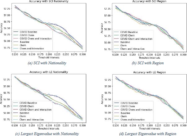
From this qualitative analysis of team chemistry in football matches onto predictions of football matches. In Fig. (4), graphs for the accuracy achieved by different prediction models are shown. 1 From these figures, the threshold interval can be determined. There is chosen symmetric threshold intervals as these are more convenient to use. To determine which threshold interval is optimal to use is not straightforward. It usually holds that the smaller the threshold interval, the higher the accuracy. All subfigures in Fig. (4) support this statement. The trend is downwards, which means the closer the threshold values to zero (the smaller the threshold interval), the higher the accuracy. However, predictions should be representative. The smaller the threshold interval, the fewer draws are predicted. Therefore the range of the threshold intervals is chosen to be between 0.1 and 0.3. Here the prediction models still perform well in terms of accuracy and predict a reasonable number of draws. In this section, the performance of two baseline prediction models will be compared to prediction models with the different chemistry measures and possible interaction effects included (chemistry models). The accuracies in Fig. (4) are calculated with 5-fold cross-validation. The confusion matrices are calculated based on one of the five folds from the cross-validation. The prediction model is estimated from 80% (35733 matches) of the data and then applied to the remaining 20% (8933 matches) to get predictions. Then these predictions are compared to the actual outcomes of the remaining 20% and the confusion matrix can be constructed. In Fig. (4a-4c), it is clear that the baseline models outperform the chemistry models with chemistry based on nationality for threshold intervals of (-0.2,0.2) and bigger, although the difference becomes smaller when the interval gets close to (-0.3,0.3). For the intervals between (-0.1,0.1) and (-0.2,0.2), the baseline models and the chemistry models do not differ much in performance on accuracy. Including chemistry based on nationality in the prediction model does not improve the model’s performance, but it could, for smaller threshold intervals, be of interest in predicting football matches. In Fig. (4b and 4d) a different story displays itself. All different models have very similar performance and the chemistry models even sometimes outperform the baseline models. The chemistry models based on the region with interaction effects with position and COVID taken into account perform outstandingly for threshold intervals up to (-0.2,0.2). For chemistry based on region and calculated with both the SCI and the largest eigenvalue method, the accuracy is the largest compared to the other models. The red lines indicating these models are the highest for most of the threshold intervals researched. The other models also perform quite well and to eventually call one of the six the best would be rash. Still, the chemistry models, for a large part, outperform the baseline models with chemistry based on region. Including these chemistry measures in prediction models can help improve the performance of predictions. To show how a threshold interval is chosen, the confusion matrices for the models with ’optimal’ threshold intervals of (Fig. 4b) will be displayed below. In Fig. (4) the purple (baseline) and blue (COVID baseline) lines show the performance of the baseline models over different threshold intervals. After investigating closely for the baseline model, a threshold interval of (-0.21,0.21) is chosen. Since the accuracy increases in comparison with a slightly smaller threshold interval of (-0.2,0.2) and decreases with a slightly bigger threshold interval of (-0.22,0.22), this is a local maximum. For smaller intervals, the accuracy increases, but the number of predicted draws decreases. Since the number of predicted draws is 1570 (17.6%) and the actual number of draws is 2147 (24.0%), this interval is chosen as the optimal one. Draws are
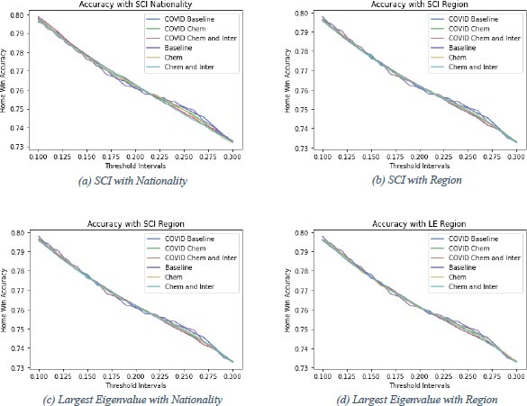
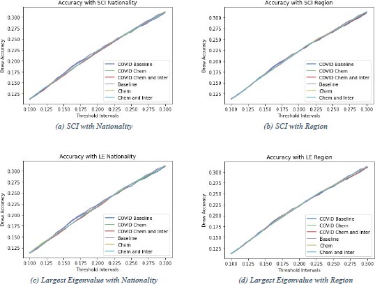
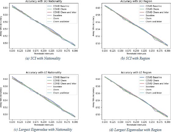
The model that is used for predictions is smaller than in the Estimation section as the accuracy become too low if all control variables are used in the prediction model. In the prediction model only a constant term and Home and Away Position are added as control variables. A Two-Way Fixed Effects model without country dummies is used for the predictions. somewhat underrepresented in the predictions but not too dramatically. The corresponding accuracy for this test set is (1551+475+3067)/8933 = 0.570 (Table 11 or 57.0%. For the COVID baseline model, a threshold interval of (-0.2,0.2) is chosen as there is a local maximum. Moreover, the number of draws that are forecast using this threshold interval is 1521 (17.0%), while the actual number of draws is 2147 (24.0%). Again, draws are somewhat underrepresented. The difference is not too drastic so this interval is chosen as the optimal one in this case and achieves an accuracy of (1568+459+3074)/8933 = 0.571 (Table 12) or 57.1% on the used test set. For the chemistry models, the chemistry measure based on region and calculated with the SCI is used. In Fig. (4b), the yellow line shows the baseline model with chemistry added to it. The yellow line first decreases fast and then almost stops decreasing to decrease faster. In this segment of - almost - no decrease, the optimal value can be found as there the accuracy does not suffer too much from choosing a wider threshold interval. The threshold interval used is (-0.21,0.21). The number of predicted draws is 1561 (17.5%), whereas there are actually 2147 (24.0%) draws. There are not too few draws and still, a reasonable accuracy of (1550+477+3072)/8933 = 0.571 (Table 13) or 57.1% is achieved on the test set. The green line represents the model when adding COVID to the model used to get the yellow line discussed above. The optimal threshold interval of (-0.19,0.19) is a local maximum. Using this threshold interval on the test set leads to an accuracy of (1581+443+3087)/8933 = 0.572 (Table 14) or 57.2%. The number of predicted draws is 1442 (16.1%), which is somewhat lower than the 2147 (24.0%) actual draws. Still, this seems to be the optimal interval to use. The chemistry models can be extended by including the interaction effect of chemistry with the position for both the home and away teams in the model. The confusion matrix of these models with the optimal threshold intervals is in table 15 and 16. The optimal threshold interval for the chemistry model without COVID, but with interaction effects included and chemistry based on region and calculated with the SCI, is (-0.2,0.2). The light blue line represents this model in Fig. (4b) and the chosen interval is a local maximum. The predicted number of draws is 1491 (16.7%), while the actual number of draws is 2147 (24.0%). The predicted number of draws is too low, but still enough to call it a realistic prediction. The model achieves an accuracy of (1572+455+3081)/8933 = 0.572 (Table 15) or 57.2%. The red line in Fig. (4b) represents the model after adding COVID. There is no local maximum, but there is a segment of almost no decrease and there, the threshold interval is optimal. This happens right before a sharp decay of the curve at 0.22. The optimal threshold interval is thus (-0.22,0.22). For this interval, the number of predicted draws on the test set is 1621 (18.1%), while the number of actual draws in the test set is 2147 (24.0%). Draws are underrepresented but not enough to throw this prediction interval away. The accuracy achieved on the test set is 1545+504+3062 8933 = 0.572 (Table 16) or 57.2%. What strikes attention from table 11-16 is that home wins are predicted quite accurately. For example, in Table 16 the number of accurately predicted home wins is 3062 or 75.3%. The number of accurately predicted away wins is 1545 or 56.8% and still reasonable. The number of accurately predicted draws is just 504 or 23.5%. Moreover, as mentioned, the number of predicted draws is just 1621 (18.1%) in this case, whereas there are actually 2147 (24.0%). As can be seen, the number of predicted home wins (4757 or 53.3%) is much bigger than the number of actual home wins (4066 or 45.5%). In contrast, the predicted number of away wins and the actual number of away wins are comparable, 2555 or 28.6% predicted versus 2720 or 30.4% actual. To get rid of this imbalance, the threshold interval for this specific example has been altered. The confusion matrix in Table 16 suggests that the number of predicted home wins should be reduced in favor of draws. With this in mind, the threshold value is changed. By trial and error, an upper bound of the interval of 0.44 has been found to predict the most comparable amount of home wins. The number of away wins was, however, too low, so the lower bound is moved up to produce a balanced prediction. Once again, by trial and error, the lower bound for the threshold interval in this example is established to be -0.17. This interval gives the confusion matrix in Table 17. As can be seen in the table, the number of predicted home wins (4082 or 45.7%), draws (2149 or 24.1%) and away wins (2702 or 30.2%) are approximately equal to the number of actual home wins (4066 or 45.5%), draws (2147 or 24.0%) and away wins (2720 or 30.4%). The percentages of the actual number of home wins, draws and away wins add up to 99.9% due to rounding. The number of accurately predicted home wins is 2745 or 67.5%, the number of accurately predicted away wins is 1607 or 59.1% and the number of accurately predicted draws is 650 or 30.3%. The asymmetric interval has made the predictions more realistic, although the prediction of draws is still challenging. An accuracy of (1607+650+2745)/8933 = 0.560 or 56.0%. This is a tiny bit lower than the accuracy achieved with the symmetric interval (-0.22,0.22) of 57.2% and illustrates the problem that is faced. An asymmetric threshold interval gives more realistic predictions but is outperformed by symmetric intervals that give slightly less realistic predictions. Finding the optimal asymmetric threshold interval is an interesting subject that can be studied in further research. As can be read off table 11-16 there is an obvious difference between predicting home wins, draws and away wins. The models seem to be comfortable predicting home wins with around 75% of the actual home wins that the prediction models correctly predict. Away win prediction is somewhat more difficult for the models, but still, approximately 57% of the actual away wins are correctly predicted by the prediction models. The models struggle clearly with predicting draws, with just roughly 21% of the draws being predicted correctly by the prediction models. Even with fine-tuning of the threshold interval, just 30.3% of the draws are predicted correctly by the prediction models. As accuracy is a weighted average of those percentages, the models can perform very differently in terms of predicting a certain outcome. This is checked by creating accuracy graphs for the three different outcomes (Figs. 5, 6, 7 and 8). From the figures, there are, apart from some small differences, no clear differences in specific outcome forecasting. This means that regarding the outcome, the models perform similarly in terms of predicting specific outcomes. There is no considerable difference between the chemistry measures either. However, the (b) and (d) parts of (Figs. 5-7) suggest that the region chemistry measures perform slightly better than the chemistry measures based on nationality. The lines representing the chemistry models lie a little higher relative to the baseline models with the region chemistry models than the nationality chemistry models. This is confirmed when these lines are summed up according to their weights in Fig. (4) where the region chemistry models clearly outperform the nationality chemistry models.
| - | COVID | SCI | SCI | LE | LE | SCI Region | SCI Region | LE Region | LE Region |
|---|---|---|---|---|---|---|---|---|---|
| - | Baseline | - | Interaction | - | Interaction | - | Interaction | - | Interaction |
| - | - | - | with position | - | with position | - | with position | - | with position |
| Home Chemistry | - | -0.0076 | 0.1170 | -0.0051 | 0.0994 | -0.0456 | 0.0514 | -0.0263 | 0.1140 |
| - | - | (0.0682) | (0.1333) | (0.0685) | (0.1342) | (0.0696) | (0.1251) | (0.0776) | (0.1496) |
| Away Chemistry | - | 0.2352 *** | 0.3869 *** | 0.2475 *** | 0.4195 *** | 0.1168 ** | -0.2004 ** | 0.0870 | -0.2349 ** |
| - | - | (0.0596) | (0.1267) | (0.0596) | (0.1267) | (0.0545) | (0.0937) | (0.0652) | (0.1069) |
| COVID | -0.0611 * | -0.0591 * | -0.0575 | -0.0586 * | -0.0573 | -0.0608 * | -0.0608 * | -0.0609 * | -0.0604 * |
| No Attendance | (0.0356) | (0.0354) | (0.0352) | (0.0353) | (0.0351) | (0.0355) | (0.0355) | (0.0356) | (0.0357) |
| Home Chemistry x | - | - | -0.0131 | - | -0.0115 | - | -0.0107 | - | -0.0159 |
| Home Position | - | - | (0.0109) | - | (0.0109) | - | (0.0101) | - | (0.0124) |
| Away Chemistry x | - | - | -0.0153 | - | -0.0181 | - | 0.0334 *** | - | 0.0340 *** |
| Away position | - | - | (0.0127) | - | (0.0121) | - | (0.0077) | - | (0.0085) |
| Home Position | -0.1007 *** | -0.1007 *** | -0.0971 *** | -0.1008 *** | -0.0951 *** | -0.1007 *** | -0.0939 *** | -0.1007 *** | -0.0888 *** |
| - | (0.0033) | (0.0033) | (0.0041) | (0.0033) | (0.0059) | (0.0033) | (0.0070) | (0.0033) | (0.0095) |
| Away Position | 0.1213 *** | 0.1202 *** | 0.1240 *** | 0.1201 *** | 0.1286 *** | 0.1211 *** | 0.1023 *** | 0.1212 *** | 0.0969 *** |
| - | (0.0024) | (0.0023) | (0.0036) | (0.0024) | (0.0057) | (0.0024) | (0.0044) | (0.0024) | (0.0058) |
| Home Height | 0.0163 *** | 0.0169 *** | 0.0167 *** | 0.0169 *** | 0.0167 *** | 0.0163 *** | 0.0161 *** | 0.0162 *** | 0.0160 *** |
| - | (0.0061) | (0.0061) | (0.0062) | (0.0061) | (0.0062) | (0.0061) | (0.0061) | (0.0062) | (0.0062) |
| Away Height | -0.0116 * | -0.0114 * | -0.0118 * | -0.0116 * | -0.0122 ** | -0.0132 ** | -0.0125 ** | -0.0126 ** | -0.0120 * |
| - | (0.0060) | (0.0060) | (0.0060) | (0.0060) | (0.0061) | (0.0061) | (0.0061) | (0.0062) | (0.0061) |
| Home Age | 0.0152 ** | 0.0168 ** | 0.0174 ** | 0.0169 ** | 0.0174 ** | 0.0154 ** | 0.0155 ** | 0.0154 ** | 0.0156 ** |
| - | (0.0073) | (0.0073) | (0.0074) | (0.0073) | (0.0074) | (0.0074) | (0.0075) | (0.0075) | (0.0075) |
| Away Age | -0.0273 *** | -0.0269 *** | -0.0264 *** | -0.0268 *** | -0.0261 *** | -0.0266 *** | -0.0277 *** | -0.0268 *** | -0.0279 *** |
| - | (0.0077) | (0.0076) | (0.0077) | (0.0076) | (0.0078) | (0.0077) | (0.0077) | (0.0077) | (0.0077) |
| Constant | -0.3994 | -0.6519 | -0.6393 | -0.6878 | -0.7028 | -0.1811 | -0.1261 | -0.2540 | -0.1881 |
| - | (1.5695) | (1.5768) | (1.5790) | (1.5722) | (1.5714) | (1.5733) | (1.5678) | (1.5770) | (1.5659) |
| R 2 | 0.1958 | 0.1962 | 0.1963 | 0.1962 | 0.1963 | 0.1959 | 0.1963 | 0.1958 | 0.1962 |
| Nr. of matches | 44666 | 44666 | 44666 | 44666 | 44666 | 44666 | 44666 | 44666 | 44666 |
5. DISCUSSION
In the Results section, a lot of interesting findings are done. Both the chemistry measures and a COVID dummy have been evaluated in estimation and prediction models. The chemistry measures used in this research seem to have a counter-intuitive effect on the outcome of a game. The hypothesis of a positive effect on performance from chemistry comes true when the chemistry is based on region and interaction effects with the position are included in the regression. The hypothesis is only valid for, at most, the top half teams, which indicates that having chemistry is only of interest when the team is already of high quality. Another explanation for this is that the measure for chemistry is not - entirely - correct. Later in this section, other ways to measure chemistry are proposed to explore in further research. As discussed in the Literature Review many factors influence chemistry within a team [13]. The insignificance of most of the estimates of Home Chemistry can be explained by the support teams get when playing at home. According to Gershgoren et al. [13], this support is part of a team’s chemistry and can have a substantial weight in the total chemistry. This means the chemistry based on connections through nationality or region has a small weight and the estimates have no significant impact. Regarding the estimates of Away Chemistry, in cases where the chemistry measure is based on nationality, the estimates are all positive and significant. This is possibly caused by the correlation of Chemistry with Position. There is a, say it small, positive correlation between the Chemistry measures based on nationality and Position. As argued in the No COVID section, lower-ranked teams often have limited resources and need to use more players from their own academy and thus have more players with the same nationality. This leads to the correlation between chemistry and position and it can thus be that the estimate of Away Chemistry measures this indirect effect on a team’s ability. COVID has the effect that is hypothesised. In all estimations, the COVID dummy has a negative sign which means that the goal difference ’moves’ in favour of the away team for matches played in empty stadiums (due to COVID). It must be noted that the estimates for COVID are often weakly or *-significant (p-value between 0.05 and 0.1) or, on a few occasions, even insignificant (p-value above 0.1). Still, the sign of the estimate of the COVID dummy is consistently negative and, most of the time, significant. To conclude, empty stadiums due to COVID decrease home advantage. The Predictions section evaluates the inclusion of chemistry, chemistry with interaction effects and COVID in prediction models. With sensible chosen symmetric threshold intervals, the accuracy of prediction models with and without the to-be-evaluated variables is measured. Including COVID does not cause any downfall in prediction accuracy, which means the inclusion of COVID will give more information to the prediction. The inclusion of the chemistry measures based on nationality does decrease prediction accuracy for a set of threshold (symmetric intervals between (-0.2,0.2) and (-0.3,0.3)) intervals and has approximately the same prediction accuracy for other threshold intervals. Prediction models, including chemistry measures based on region, do on occasion, outperform baseline models and are certainly not systematically outperformed by these baseline models. In conclusion, including COVID and chemistry in predictions does not necessarily improve predictions as is hypothesised. The inclusion of COVID and chemistry measures based on region is, however, highly recommended as prediction performance does not decrease and information increases. Fine-tuning these threshold intervals is interesting to explore in further research. The intervals can, for example, be based on the minimized prediction error or determined by an extensive grid search with cross-validation. This research contributes to the field of football analysis by studying the effect of team chemistry on the outcome of football matches and the inclusion of chemistry in football prediction models. In combination with the incorporation of COVID, this research provides a unique perspective on football research which can be elaborated on in future research.
6. CHEMISTRY IN FUTURE RESEARCH
As the measures used in this research only consider nationality and region to cause chemistry and only consider two methods to calculate it, there is a lot to explore in this area. In further research, measures based on different or multiple factors and different calculation methods such as a weighted SCI or a combination of both nationality and region can lead to better chemistry measures and more informative estimation and prediction results. Some ideas to base the chemistry measure on in the future will be listed below. Base connections on the language players speak rather than nationality as a player can speak multiple languages this is more inclusive. There are just eight regions that the world is split into in this research. Dividing the world into smaller regions, for example, the United Kingdom, Benelux and the Iberian Peninsula. Furthermore, giving weight to the connections between countries can improve the measure drastically. However, this would mean first, the number of nationalities squared connections between the different countries need to be found. Differencing between countrymen who play in their own country and those who play in a different country can also provide a direction in which chemistry can be improved. Connections between countrymen that play abroad are often quite strong [26, 27]. Connections can also be based on the number of matches players have played together previously. Another possibility is to weigh the players according to how long they play in a match. Combining and weighting the nationality and region connections can provide a clearer picture of chemistry. Weighting connections on the position can make the chemistry more realistic. For example, a player that plays left in defense will usually not have much to do with a right midfielder, while this left defender will be most involved with the central defender and left midfielder. Furthermore, one can also base the chemistry on something different such as height or weight or the number of matches players have played together. Combinations of all of the mentioned directions can, of course, also provide a better chemistry measure. Lastly, although there are many more possibilities, the reasoning of connections can be turned around and it can be researched how unconnected players are and create an ’inverse’ chemistry measure. This can be done with the cultural distance index [28].
CONCLUSION
These suggestions are all formed by critical thinking, and discussion with teachers and fellow master students and some are based on examples from the world of football. As it becomes clear, there are many ways in which the chemistry measure can be improved. The proposed improvements are just a fraction of all the possible measures that can be used for chemistry. Exploring these different chemistry measures is a very interesting thing that can and should be conducted in future research.
ETHICS APPROVAL AND CONSENT TO PARTICIPATE
Not applicable.
HUMAN AND ANIMAL RIGHTS
No animals/humans were used in this research.
CONSENT FOR PUBLICATION
Not applicable.
AVAILABILITY OF DATA AND MATERIALS
Not applicable.
FUNDING
None.
CONFLICT OF INTEREST
The author declares no conflict of interest, financial or otherwise.
ACKNOWLEDGEMENTS
Declared none.
APPENDIX
Robustness Checks
Robustness checks for the estimations can be found in this section. table 18 and 19 are the robustness checks for the results from the No COVID part of the results. table 20 and 21 are the robustness checks for the results from the COVID part of the results. table 22-35 is an overlapping robustness check for estimations from both parts of the result section.
| - | baseline | SCI | SCI | LE | LE |
|---|---|---|---|---|---|
| - | - | - | Interaction | - | Interaction |
| Home Chemistry | - | -0.0070 | 0.1204 | -0.0027 | 0.1044 |
| - | - | (0.0698) | (0.1400) | (0.0704) | (0.1404) |
| Away Chemistry | - | 0.1933*** | 0.3228*** | 0.2063*** | 0.3620*** |
| - | - | (0.0504) | (0.1192) | (0.0505) | (0.1195) |
| Home Chemistry x | - | - | -0.0134 | - | -0.0117 |
| Home Position | - | - | (0.0113) | - | (0.0113) |
| Away Chemistry x | - | - | -0.0131 | - | -0.0163 |
| Away Position | - | - | (0.0127) | - | (0.0120) |
| Home Position | -0.1013*** | -0.1013*** | -0.0975*** | -0.1013*** | -0.0955*** |
| - | (0.0034) | (0.0034) | (0.0042) | (0.0034) | (0.0061) |
| Away Position | 0.1214*** | 0.1205*** | 0.1237*** | 0.1204*** | 0.1281*** |
| - | (0.0024) | (0.0023) | (0.0035) | (0.0023) | (0.0056) |
| Home Height | 0.0162** | 0.0168*** | 0.0166*** | 0.0168*** | 0.0166*** |
| - | (0.0063) | (0.0063) | (0.0064) | (0.0063) | (0.0064) |
| Away Height | -0.0092 | -0.0092 | -0.0096 | -0.0093 | -0.0099* |
| - | (0.0059) | (0.0059) | (0.0059) | (0.0059) | (0.0059) |
| Home Age | 0.0158$** | 0.0171** | 0.0176** | 0.0172** | 0.0177** |
| - | (0.0072) | (0.0073) | (0.0074) | (0.0073) | (0.0074) |
| Away Age | -0.0253*** | -0.0250*** | -0.0246*** | -0.0249*** | -0.0243*** |
| - | (0.0076) | (0.0075) | (0.0076) | (0.0075) | (0.0077) |
| Constant | -1.8902 | -2.0594 | -2.0494 | -2.0951 | -2.1132 |
| - | (1.5866) | (1.5901) | (1.5919) | (1.5846) | (1.5824) |
| Ukraine | 1.7486*** | 1.6752*** | 1.6689*** | 1.6795*** | 1.6746*** |
| - | (0.2488) | (0.2455) | (0.2429) | (0.2457) | (0.2437) |
| Denmark | 1.7543*** | 1.7140*** | 1.7146*** | 1.7123*** | 1.7143*** |
| - | (0.1853) | (0.1836) | (0.1820) | (0.1813) | (0.1797) |
| Russia | 1.0761*** | 1.0474*** | 1.0488*** | 1.0420*** | 1.0447*** |
| - | (0.2679) | (0.2644) | (0.2642) | (0.2640) | (0.2637) |
| Turkey | 1.0695*** | 1.0639*** | 1.0661*** | 1.0611*** | 1.0636*** |
| - | (0.2355) | (0.2342) | (0.2344) | (0.2342) | (0.2343) |
| Belgium | 1.7839*** | 1.7866*** | 1.7917*** | 1.7856*** | 1.7911*** |
| - | (0.2274) | (0.2253) | (0.2248) | (0.2252) | (0.2250) |
| Scotland | 2.3837*** | 2.3631*** | 2.3647*** | 2.3628*** | 2.3648*** |
| - | (0.4322) | (0.4301) | (0.4312) | (0.4294) | (0.4302) |
| Greece | 1.9982*** | 1.9872*** | 1.9929*** | 1.9856*** | 1.9942*** |
| - | (0.1932) | (0.1899) | (0.1904) | (0.1894) | (0.1900) |
| Portugal | 1.1115*** | 1.0971*** | 1.0999*** | 1.0984*** | 1.1016*** |
| - | (0.1803) | (0.1773) | (0.1767) | (0.1766) | (0.1759) |
| Netherlands | 1.4149*** | 1.3983*** | 1.3999*** | 1.3950*** | 1.3985*** |
| - | (0.1216) | (0.1197) | (0.1202) | (0.1199) | (0.1209) |
| France | 0.6343*** | 0.6223*** | 0.6221*** | 0.6184*** | 0.6190*** |
| - | (0.1775) | (0.1755) | (0.1750) | (0.1752) | (0.1745) |
| Italy | 0.4845*** | 0.4812*** | 0.4859*** | 0.4820*** | 0.4891*** |
| - | (0.1513) | (0.1500) | (0.1506) | (0.1497) | (0.1505) |
| Germany | 0.3162** | 0.3082** | 0.3109** | 0.3045** | 0.3082** |
| - | (0.1558) | (0.1550) | (0.1549) | (0.1551) | (0.1550) |
| Spain | 0.3225** | 0.2871* | 0.2918* | 0.2851* | 0.2915* |
| - | (0.1601) | (0.1599) | (0.1601) | (0.1590) | (0.1592) |
| Europe | 0.7143*** | 0.7028*** | 0.7075*** | 0.7026*** | 0.7090*** |
| - | (0.1304) | (0.1288) | (0.1284) | (0.1285) | (0.1282) |
| R2 | 0.2024 | 0.2027 | 0.2027 | 0.2027 | 0.2028 |
| N | 44666 | 44666 | 44666 | 44666 | 44666 |
| - | SCI | SCI | LE | LE |
|---|---|---|---|---|
| - | - | Interaction | - | Interaction |
| Home Chemistry | -0.0582 | 0.0356 | -0.0411 | 0.0959 |
| - | (0.0714) | (0.1302) | (0.0799) | (0.1558) |
| Away Chemistry | 0.0995* | -0.2308** | 0.0759 | -0.2644** |
| - | (0.0511) | (0.0900) | (0.0621) | (0.1037) |
| Home Chemistry x | - | -0.0103 | - | -0.0155 |
| Home Position | - | (0.0105) | - | (0.0129) |
| Away Chemistry x | - | 0.0347*** | - | 0.0359*** |
| Away Position | - | (0.0077) | - | (0.0085) |
| Home Position | -0.1013*** | -0.0947*** | -0.1013*** | -0.0896*** |
| - | (0.0034) | (0.0072) | (0.0034) | (0.0099) |
| Away Position | 0.1212*** | 0.1016*** | 0.1213*** | 0.0957*** |
| - | (0.0023) | (0.0043) | (0.0023) | (0.0057) |
| Home Height | 0.0165** | 0.0163** | 0.0164** | 0.0161** |
| - | (0.0064) | (0.0064) | (0.0064) | (0.0064) |
| Away Height | -0.0105* | -0.0097 | -0.0100* | -0.0093 |
| - | (0.0060) | (0.0060) | (0.0060) | (0.0060) |
| Home Age | 0.0157** | 0.0158** | 0.0158** | 0.0160** |
| - | (0.0074) | (0.0074) | (0.0074) | (0.0074) |
| Away Age | -0.0248*** | -0.0260*** | -0.0249*** | -0.0262*** |
| - | (0.0076) | (0.0076) | (0.0076) | (0.0076) |
| Constant | -1.7467 | -1.6937 | -1.7962 | -1.7256 |
| - | (1.5971) | (1.5925) | (1.6037) | (1.5917) |
| Ukraine | 1.7313*** | 1.7519*** | 1.7402*** | 1.7565*** |
| - | (0.2481) | (0.2493) | (0.2489) | (0.2502) |
| Denmark | 1.7432*** | 1.7600*** | 1.7493*** | 1.7607*** |
| - | (0.1849) | (0.1854) | (0.1851) | (0.1864) |
| Russia | 1.0689*** | 1.0664*** | 1.0728*** | 1.0728*** |
| - | (0.2672) | (0.2679) | (0.2678) | (0.2689) |
| Turkey | 1.0941*** | 1.1040*** | 1.0878*** | 1.1002*** |
| - | (0.2348) | (0.2375) | (0.2331) | (0.2363) |
| Belgium | 1.7955*** | 1.7833*** | 1.7922*** | 1.7838*** |
| - | (0.2276) | (0.2286) | (0.2274) | (0.2276) |
| Scotland | 2.3700*** | 2.3882*** | 2.3763*** | 2.3946*** |
| - | (0.4328) | (0.4312) | (0.4334) | (0.4306) |
| Greece | 2.0001*** | 2.0003*** | 2.0003*** | 2.0003*** |
| - | (0.1918) | (0.1964) | (0.1924) | (0.1961) |
| Portugal | 1.1307*** | 1.1323*** | 1.1262*** | 1.1288*** |
| - | (0.1800) | (0.1845) | (0.1815) | (0.1850) |
| Netherlands | 1.4181*** | 1.4099*** | 1.4171*** | 1.4099*** |
| - | (0.1219) | (0.1216) | (0.1219) | (0.1212) |
| France | 0.6482*** | 0.6530*** | 0.6453*** | 0.6506*** |
| - | (0.1774) | (0.1793) | (0.1775) | (0.1790) |
| Italy | 0.4874*** | 0.4870*** | 0.4874*** | 0.4867*** |
| - | (0.1510) | (0.1541) | (0.1509) | (0.1533) |
| Germany | 0.3121** | 0.3210** | 0.3139** | 0.3207** |
| - | (0.1548) | (0.1583) | (0.1555) | (0.1582) |
| Spain | 0.3249** | 0.3265** | 0.3250** | 0.3256** |
| - | (0.1595) | (0.1618) | (0.1598) | (0.1615) |
| Europe | 0.7184*** | 0.7201*** | 0.7180*** | 0.7200*** |
| - | (0.1302) | (0.1325) | (0.1303) | (0.1322) |
| R2 | 0.2025 | 0.2029 | 0.2024 | 0.2028 |
| N | 44666 | 44666 | 44666 | 44666 |
Table 20.
| - | baseline | SCI | SCI | LE | LE |
|---|---|---|---|---|---|
| - | - | - | Interaction | - | Interaction |
| Home Chemistry | - | -0.0090 | 0.1168 | -0.0052 | 0.1009 |
| - | - | (0.0697) | (0.1396) | (0.0704) | (0.1401) |
| Away Chemistry | - | 0.1925*** | 0.3196*** | 0.2053*** | 0.3594*** |
| - | - | (0.0505) | (0.1193) | (0.0504) | (0.1195) |
| COVID/ | -0.0650* | -0.0635* | -0.0622* | -0.0631* | -0.0620* |
| No Attendance | (0.0349) | (0.0348) | (0.0346) | (0.0347) | (0.0346) |
| Home Chemistry x | - | - | -0.0132 | - | -0.0116 |
| Home Position | - | - | (0.0113) | - | (0.0113) |
| Away Chemistry x | - | - | -0.0128 | - | -0.0162 |
| Away Position | - | - | (0.0127) | - | (0.0120) |
| Home Position | -0.1012*** | -0.1012*** | -0.0975*** | -0.1012*** | -0.0954*** |
| - | (0.0034) | (0.0034) | (0.0042) | (0.0034) | (0.0061) |
| Away Position | 0.1215*** | 0.1206*** | 0.1237*** | 0.1205*** | 0.1281*** |
| - | (0.0024) | (0.0023) | (0.0035) | (0.0023) | (0.0056) |
| Home Height | 0.0160** | 0.0166*** | 0.0164*** | 0.0166*** | 0.0164** |
| - | (0.0063) | (0.0063) | (0.0063) | (0.0063) | (0.0064) |
| Away Height | -0.0093 | -0.0093 | -0.0096 | -0.0094 | -0.0099* |
| - | (0.0059) | (0.0059) | (0.0059) | (0.0059) | (0.0059) |
| Home Age | 0.0158** | 0.0171** | 0.0176** | 0.0172** | 0.0177** |
| - | (0.0072) | (0.0073) | (0.0073) | (0.0073) | (0.0074) |
| Away Age | -0.0254*** | -0.0251*** | -0.0247*** | -0.0250*** | -0.0244*** |
| - | (0.0076) | (0.0075) | (0.0076) | (0.0076) | (0.0077) |
| Constant | -1.8320 | -1.9990 | -1.9905 | -2.0340 | -2.0530 |
| - | (1.5852) | (1.5881) | (1.5898) | (1.5826) | (1.5801) |
| Ukraine | 1.7476*** | 1.6746*** | 1.6684*** | 1.6789*** | 1.6740*** |
| - | (0.2493) | (0.2460) | (0.2433) | (0.2462) | (0.2441) |
| Denmark | 1.7507*** | 1.7107*** | 1.7113*** | 1.7090*** | 1.7111*** |
| - | (0.1858) | (0.1841) | (0.1825) | (0.1818) | (0.1803) |
| Russia | 1.0714*** | 1.0430*** | 1.0444*** | 1.0376*** | 1.0404*** |
| - | (0.2668) | (0.2634) | (0.2632) | (0.2630) | (0.2627) |
| Turkey | 1.0762*** | 1.0705*** | 1.0725*** | 1.0677*** | 1.0701*** |
| - | (0.2361) | (0.2349) | (0.2350) | (0.2348) | (0.2349) |
| Belgium | 1.7812*** | 1.7839*** | 1.7890*** | 1.7830*** | 1.7885*** |
| - | (0.2275) | (0.2254) | (0.2249) | (0.2254) | (0.2251) |
| Scotland | 2.3816*** | 2.3612*** | 2.3628*** | 2.3609*** | 2.3629*** |
| - | (0.4322) | (0.4301) | (0.4311) | (0.4294) | (0.4302) |
| Greece | 2.0065*** | 1.9953*** | 2.0008*** | 1.9937*** | 2.0021*** |
| - | (0.1945) | (0.1913) | (0.1918) | (0.1908) | (0.1914) |
| Portugal | 1.1133*** | 1.0989*** | 1.1016*** | 1.1002*** | 1.1033*** |
| - | (0.1798) | (0.1768) | (0.1762) | (0.1761) | (0.1754) |
| Netherlands | 1.4150*** | 1.3985*** | 1.4001*** | 1.3952*** | 1.3986*** |
| - | (0.1213) | (0.1195) | (0.1200) | (0.1196) | (0.1207) |
| France | 0.6304*** | 0.6184*** | 0.6184*** | 0.6146*** | 0.6153*** |
| - | (0.1764) | (0.1744) | (0.1739) | (0.1741) | (0.1734) |
| Italy | 0.4831*** | 0.4799*** | 0.4845*** | 0.4807*** | 0.4877*** |
| - | (0.1513) | (0.1499) | (0.1505) | (0.1497) | (0.1504) |
| Germany | 0.3153** | 0.3073** | 0.3100** | 0.3036* | 0.3074** |
| - | (0.1558) | (0.1549) | (0.1549) | (0.1551) | (0.1549) |
| Spain | 0.3225** | 0.2872* | 0.2918* | 0.2853* | 0.2915* |
| - | (0.1600) | (0.1598) | (0.1600) | (0.1590) | (0.1592) |
| Europe | 0.7145*** | 0.7031*** | 0.7076*** | 0.7028*** | 0.7092*** |
| - | (0.1305) | (0.1289) | (0.1285) | (0.1286) | (0.1283) |
| R2 | 0.2025 | 0.2027 | 0.2028 | 0.2027 | 0.2028 |
| N | 44666 | 44666 | 44666 | 44666 | 44666 |
| - | SCI | SCI | LE | LE |
|---|---|---|---|---|
| - | - | Interaction | - | Interaction |
| Home Chemistry | -0.0585 | 0.0358 | -0.0414 | 0.0965 |
| - | (0.0714) | (0.1300) | (0.0799) | (0.1554) |
| Away Chemistry | 0.0994* | -0.2306** | 0.0759 | -0.2634** |
| - | (0.0511) | (0.0902) | (0.0622) | (0.1038) |
| COVID/ | -0.0650* | -0.0649* | -0.0650* | -0.0644* |
| No Attendance | (0.0347) | (0.0347) | (0.0348) | (0.0349) |
| Home Chemistry x | - | -0.0104 | - | -0.0156 |
| Home Position | - | (0.0105) | - | (0.0128) |
| Away Chemistry x | - | 0.0346*** | - | 0.0358*** |
| Away Position | - | (0.0077) | - | (0.0085) |
| Home Position | -0.1012*** | -0.0945*** | -0.1012*** | -0.0894*** |
| - | (0.0033) | (0.0072) | (0.0034) | (0.0098) |
| Away Position | 0.1213*** | 0.1017*** | 0.1214*** | 0.0959*** |
| - | (0.0023) | (0.0043) | (0.0023) | (0.0057) |
| Home Height | 0.0163** | 0.0161** | 0.0162** | 0.0159** |
| - | (0.0064) | (0.0064) | (0.0064) | (0.0064) |
| Away Height | -0.0105* | -0.0098 | -0.0101* | -0.0094 |
| - | (0.0060) | (0.0060) | (0.0060) | (0.0060) |
| Home Age | 0.0157** | 0.0158** | 0.0158** | 0.0160** |
| - | (0.0073) | (0.0074) | (0.0074) | (0.0074) |
| Away Age | -0.0249*** | -0.0261*** | -0.0250*** | -0.0263*** |
| - | (0.0076) | (0.0077) | (0.0076) | (0.0076) |
| Constant | -1.6893 | -1.6367 | -1.7385 | -1.6695 |
| - | (1.5965) | (1.5918) | (1.6029) | (1.5909) |
| Ukraine | 1.7304*** | 1.7510*** | 1.7392*** | 1.7556*** |
| - | (0.2486) | (0.2497) | (0.2494) | (0.2507) |
| Denmark | 1.7396*** | 1.7564*** | 1.7457*** | 1.7571*** |
| - | (0.1853) | (0.1858) | (0.1856) | (0.1869) |
| Russia | 1.0642*** | 1.0617*** | 1.0680*** | 1.0681*** |
| - | (0.2661) | (0.2668) | (0.2667) | (0.2678) |
| Turkey | 1.1009*** | 1.1107*** | 1.0945*** | 1.1069*** |
| - | (0.2354) | (0.2381) | (0.2337) | (0.2370) |
| Belgium | 1.7928*** | 1.7806*** | 1.7895*** | 1.7812*** |
| - | (0.2277) | (0.2287) | (0.2275) | (0.2277) |
| Scotland | 2.3680*** | 2.3862*** | 2.3742*** | 2.3925*** |
| - | (0.4328) | (0.4312) | (0.4334) | (0.4306) |
| Greece | 2.0084*** | 2.0086*** | 2.0087*** | 2.0086*** |
| - | (0.1932) | (0.1978) | (0.1938) | (0.1974) |
| Portugal | 1.1325*** | 1.1341*** | 1.1280*** | 1.1306*** |
| - | (0.1795) | (0.1840) | (0.1810) | (0.1845) |
| Netherlands | 1.4183*** | 1.4101*** | 1.4172*** | 1.4101*** |
| - | (0.1216) | (0.1213) | (0.1216) | (0.1209) |
| France | 0.6442*** | 0.6490*** | 0.6414*** | 0.6467*** |
| - | (0.1762) | (0.1781) | (0.1764) | (0.1778) |
| Italy | 0.4860*** | 0.4856*** | 0.4860*** | 0.4854*** |
| - | (0.1509) | (0.1541) | (0.1509) | (0.1532) |
| Germany | 0.3112** | 0.3201** | 0.3130** | 0.3198** |
| - | (0.1548) | (0.1583) | (0.1554) | (0.1582) |
| Spain | 0.3249** | 0.3265** | 0.3249** | 0.3256** |
| - | (0.1594) | (0.1617) | (0.1597) | (0.1614) |
| Europe | 0.7186*** | 0.7204*** | 0.7183*** | 0.7202*** |
| - | (0.1303) | (0.1325) | (0.1304) | (0.1323) |
| R2 | 0.2025 | 0.2030 | 0.2025 | 0.2029 |
| N | 44666 | 44666 | 44666 | 44666 |
| - | baseline | SCI Region | SCI Region | COVID | SCI Region | SCI Region |
|---|---|---|---|---|---|---|
| - | - | - | - | baseline | COVID | COVID |
| - | - | - | Interaction | - | - | Interaction |
| - | - | - | with position | - | - | with position |
| Home Chemistry | - | -0.0607 | 0.0329 | - | -0.0608 | 0.0334 |
| - | - | (0.060) | (0.082) | - | (0.060) | (0.082) |
| Away Chemistry | - | 0.0791 | -0.1160 | - | 0.0790 | -0.1169 |
| - | - | (0.060) | (0.104) | - | (0.060) | (0.104) |
| COVID/ | - | - | - | -0.0731** | -0.0731** | -0.0739** |
| No Attendance | - | - | - | (0.037) | (0.037) | (0.037) |
| Home Chemistry x | - | - | -0.0103* | - | - | -0.0104* |
| Home Position | - | - | (0.006) | - | - | (0.006) |
| Away Chemistry x | - | - | 0.0212** | - | - | 0.0212** |
| Away Position | - | - | (0.009) | - | - | (0.009) |
| Home Position | -0.1035*** | -0.1035*** | -0.0969*** | -0.1034*** | -0.1034*** | -0.0967*** |
| - | (0.002) | (0.002) | (0.004) | (0.002) | (0.002) | (0.004) |
| Away Position | 0.0981*** | 0.0981*** | 0.0862*** | 0.0981*** | 0.0981*** | 0.0862*** |
| - | (0.002) | (0.002) | (0.006) | (0.002) | (0.002) | (0.006) |
| Home Height | 0.0193*** | 0.0197*** | 0.0196*** | 0.0191*** | 0.0195*** | 0.0194*** |
| - | (0.006) | (0.006) | (0.006) | (0.006) | (0.006) | (0.006) |
| Away Height | -0.0235*** | -0.0242*** | -0.0240*** | -0.0236*** | -0.0243*** | -0.0241*** |
| - | (0.006) | (0.006) | (0.006) | (0.006) | (0.006) | (0.006) |
| Home Age | 0.0221*** | 0.0219*** | 0.0220*** | 0.0220*** | 0.0218*** | 0.0219*** |
| - | (0.007) | (0.007) | (0.007) | (0.007) | (0.007) | (0.007) |
| Away Age | -0.0356*** | -0.0351*** | -0.0358*** | -0.0357*** | -0.0352*** | -0.0359*** |
| - | (0.007) | (0.007) | (0.007) | (0.007) | (0.007) | (0.007) |
| Constant | 1.4495 | 1.4870 | 1.5344 | 1.5215 | 1.5587 | 1.6067 |
| - | (1.503) | (1.508) | (1.508) | (1.503) | (1.508) | (1.509) |
| R2 | 0.319 | 0.319 | 0.319 | 0.319 | 0.319 | 0.319 |
| Nr. of parameters | 843 | 845 | 847 | 844 | 846 | 848 |
| Nr. of matches | 44666 | 44666 | 44666 | 44666 | 44666 | 44666 |
Dataset
Creating the Dataset
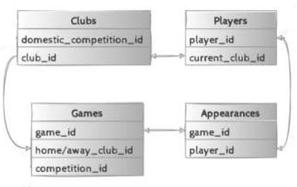
The final dataset is created by merging four datasets. One club dataset, one players dataset, one games dataset and one appearance dataset. Every game has a game_id. If a player makes an appearance in a game this appearance is also given a game_id through which these datasets are linked. Then to know which players actually play the appearance consists also of a player_id. This player_id is linked to the players dataset in which each player has a player_id. The players play for a certain club and these clubs have a club_id that can be found in the games dataset that contains the club_id of both the home and away team. This completes the circle and with python these datasets are merged and the final dataset that is used in this research is created.
Region
The world is split up into eight regions in this research to measure connections between players. These regions are used for two of the four proposed chemistry measures. The eight regions are Europe, Africa, South America, Middle East, North and Central America, Asia, Caribbean and Oceania. The countries that are part of these regions will be listed below. It should be mentioned that not all countries of the world will be in one of the regions as only countries from which at least one player comes from in the dataset are included.
The countries that fall into Europe in this research are Russia, Netherlands, Belgium, England, Northern Ireland, Ireland, France, Scotland, Spain, Czech Republic, Germany, Croatia, Serbia, Italy, Portugal, Slovakia, Hungary, Poland, Belarus, Romania, Greece, Norway, Ukraine, Estonia, Denmark, Finland, Austria, Iceland, Faroe Islands, Sweden, Albania, Switzerland, Bosnia-Herzegovina, Cyprus, Wales, Slovenia, Montenegro, Lithuania, Latvia, North Macedonia, Luxembourg, Malta, San Marino, Moldova, Armenia, Monaco, Kosovo, Liechtenstein, Andorra, Azerbaijan, Georgia and Bulgaria.
The countries that fall into Africa in this research are Cote d’Ivoire, DR Congo, Cameroon, Burkina Faso, Ghana, Uganda, Morocco, Nigeria, Sierra Leone, Algeria, Mali, Kenya, South Africa, Tunisia, Zambia, Angola, Guinea, Gabon, Mauritania, Central African Republic, Guinea-Bissau, Tanzania, Cape Verde, Madagascar, Niger, Mozambique, Congo, Gambia, Eritrea, Zimbabwe, Malawi, Chad, Sao Tome and Principe, Equatorial Guinea, Ethiopia, Somalia, Mauritius, Rwanda, Burundi, Liberia, Comoros, Togo, Benin and Senegal.
The countries that fall into Asia in this research are Thailand, China, Japan, North Korea, South Korea, Indonesia, Kazakhstan, Taiwan, Philippines, Pakistan, Uzbekistan, Vietnam, Macao, Tajikistan, Brunei Darussalam, Kyrgyzstan, Malaysia, Laos and Turkmenistan.
The countries that fall into Caribbean in this research are Guadeloupe, Trinidad and Tobago, Antigua and Barbuda, Grenada, Montserrat, Curacao, St. Kitts & Nevis, Saint-Martin, St. Lucia, Aruba, Dominican Republic, Haiti, Jamaica, Barbados, Martinique and Cuba.
The countries that fall into Middle East in this research are Egypt, Jordan, Qatar, Iran, Iraq, Israel, Syria, Turkey, Palestine, Lebanon, Saudi Arabia, Bahrain, Afghanistan and Libya.
The countries that fall into North and Central America in this research are the United States, Canada, Panama, Costa Rica, Nicaragua, Mexico, El Salvador, Bermuda and Honduras.
The countries that fall into South America in this research are Argentina, Brazil, Uruguay, Chile, Colombia, Paraguay, Ecuador, Bolivia, Peru, Suriname, Venezuela, French Guiana and Guyana.
The countries that fall into Oceania in this research are Australia, New Zealand, New Caledonia and Papua New Guinea.
Missing Values
To create the dataset there had to be dealt with missing values. For example, in a cup match there is no ranking for both teams while in a competition match there is a ranking for both teams. In cases of missing values like these, the previous value of the ranking (or another variable) of that particular team is taken. The age, height and chemistry variables are only calculated if the number of players that played for a team in a match is eleven or higher. In other cases, no value is reported and this will be dealt with as disscussed above.
Confusion Matrices
Below the confusion matrices for the predictions made by the models with chemistry based on SCI Nationality, LE Nationality and LE Region. The prediction models are estimated on a training set of 80% of the data and then the prediction is done on a test set of the remaining 20%. In all the table the same training and test set are used.
| Home Position | Away Position | |
|---|---|---|
| Home Chemistry SCI Nationality | 0.0829 | |
| Away Chemistry SCI Nationality | 0.0857 | |
| Home Chemistry LE Nationality | 0.1017 | |
| Away Chemistry LE Nationality | 0.1064 | |
| Home Chemistry SCI Region | -0.0159 | |
| Away Chemistry SCI Region | -0.0202 | |
| Home Chemistry LE Region | -0.0163 | |
| Away Chemistry LE Region | -0.0219 |
Correlations
The correlations between the chemistry measures and the position variables.