All published articles of this journal are available on ScienceDirect.

Statistical Adjustment for Tactical Choices When Evaluating Team’s Offensive Output Across Five Major European Club Soccer Leagues
Abstract
Introduction
Match statistics from the England-France 2022 FIFA World Cup Quarterfinal might suggest England lost despite playing better than France: 16 shot attempts to 8, 5 corners to 2, yet suffering a 1-2 defeat. This interpretation, however, ignores the scoring context.
Methods
During the 40 minutes, the match was tied (0-0 and 1-1), France actually led in all of the aforementioned statistical categories. Once ahead, France deliberately ceded the initiative to England for 66 minutes to protect their lead. To study the effects of tactical decisions on offensive outputs like shot attempts and corner kicks, we analyzed sequenced match event data from five major European leagues over 15 years. Our approach incorporates scoring context and other tactical drivers, such as red card differentials and home-field advantage, while controlling for team quality using pre-match betting odds. For that, we leverage modeling approaches tailored towards count response data, priori-tizing balance between quality of fit and simplicity.
Results
Our data analysis provides a thorough confirmation for several intuitive aspects of game dynamics, e.g., that leading or shorthanded teams typically produce less offense, while teams that trail or have more men tend to ramp up their attacks. Beyond this, we develop a statistical adjustment mechanism to teams’ offensive outputs that equalizes the contextual factors for both teams, helping obtain a potentially fairer representation of their relative statistical outputs within a game.
Conclusion
This analysis sheds light on how match context drives observed disparities in offensive outputs and offers an alternative, more nuanced, framework for understanding and assessing team performance.
1. INTRODUCTION
Soccer, also known as football, is one of the most popular sports in the world. According to the International Federation of Association Football (French: F´ed´eration Internationale de Football Association), approximately 5 billion people engaged with the FIFA World Cup Qatar 2022 [1].
In soccer, statistics play a crucial role in analyzing various aspects of the game, ranging from evaluating player and team performance to providing valuable strategic insights. For instance, metrics such as shot attempts and corner kicks can illustrate which team was more proactive dur-ing a match. However, relying solely on aggregate game totals without considering the specific context in which these events occurred can often lead to misinterpretation.
For instance, analyzing the match statistics from the 2022 FIFA World Cup Quarterfinal between England and France might lead one to conclude that “England lost despite being the better team,” based on having taken 16 shot attempts to France’s 8, 8 shots on target to France’s 5, and earning 5 corners to France’s 2, ultimately resulting in a 1-2 loss [2]. However, metrics derived solely from these total shot and corner counts fail to account for scoring context. During the 40 minutes when the match was tied (0-0 and 1-1), France led in all the aforementioned statistical categories. In contrast, during the 66 minutes when France was ahead, they consciously ceded initiative to England as a tactical choice to protect their lead. The goal of our work is to investigate how various contextual factors—such as score differential—affect a team’s offensive pro-duction metrics (e.g., shot attempts and corners) and adjust these numbers accordingly. Such adjustments aim to provide a more objective representation of each team’s performance within a specific game. In this section, we first introduce previous research and metrics in soccer analytics, as well as analogous research questions explored in other sports. We then conclude by detailing our specific research question and its novel contributions.
1.1. Previous Research
Existing metrics and approaches in soccer performance analysis employ a range of methodologies aimed at describing game dynamics. One of the most popular tools in modern soccer analytics is the Expected Goal (xG) model [3], which evaluates the probability of a shot resulting in a goal based on factors such as shot location, angle, distance, and type. By assigning a numerical value to the quality of scoring chances, xG models provide a quantitative measure of the quality of shots and opportunities generated by a team. Similarly, there has been research into calculating the probabilities of completing a pass (xPass) and increasing the likelihood of creating scoring opportunities by moving the ball between zones (xThreat) [4, 5]. Analogous methodologies exist in other sports. In American football, Expected Points Added (EPA) metric evaluates the contribution of each play toward scoring, accounting for game context rather than focusing solely on plays that directly result in a score [6]. Similarly, a study [7] derived the expected value of possession in rugby, incorporating contextual factors such as field location and the nature of the preceding possession’s outcome (e.g., opposition error, penalty, goal-line dropout, or completed set).
In addition to shot or pass characteristics, some models incorporate other factors as proxies to quantify psychological effects, such as match attendance, match importance, and goal differential [8]. Mead et al. suggested that psychological pressure may influence the likelihood of scoring goals, highlighting goal differential as one of the most influential variables in expected goals models. However, the precise nature of this effect was not studied in detail due to the use of overly complex, low-interpretability models, often referred to as “black box” models.
With regard to explicit statistical adjustments for contextual information in soccer, the authors [9, 10] modeled the dependence between goals scored and conceded by a team in a match using various bivariate distributions. These studies also incorporated an ”offense-defense” model [11, 12] for American football for college basketball. This model assumes that a team’s scoring output is a function of its offensive strength and the opponent’s defensive strength, thereby adjusting for the quality of the opposition. As a further extension, another study [13] analyzed American college football data to adjust several offensive statistics for both the strength of the opponent and the contributions of a subset of the team’s own players (referred to as the ”complementary unit”). Finally, acknowledging the critical role of home-field advantage [14], all the models mentioned above incorporated adjustments for the home factor.
1.2. Research Question
This paper seeks to address the limitations of traditional soccer match statistics, such as total shot attempts and corner kicks, which often overlook tactical context within the game. Using match event sequencing data from five major European leagues over the past 15 years, we examine the impacts of tactical decisions on these statistical categories (shot attempts and corner kicks). Specifically, we hypothesized that the likelihood of implementing certain tactics is associated with several factors, including the score and red card differential during a given time period, the length of that period, and whether the team is playing at home or away. Additionally, prematch betting coefficients are incorporated to measure how evenly matched the two teams are, as this is hypothesized to be a critical variable to control for when estimating the effects of the aforementioned factors on tactical decisions.
Ultimately, we study the nature of these impacts and apply a statistical adjustment to account for contextual factors. By projecting each team’s performance onto a standardized baseline scenario (a tied home game with equal number of play-ers on both teams), this adjustment aims to provide a more objective evaluation of team performance and offer novel insights into game dynamics.
Although there has been research conducted previously on modeling offensive metrics as a function of various contextual factors within a game, including score differential, our work differs in several key aspects. First, we focus on other statistical categories, such as shot attempts and corners, which also play an important role in evaluating team performance. Second, we incor-porate contextual factors, such as red card differential, and control for potential disparities in team levels using prematch betting coefficients—both of which, to the best of our knowledge, have not been addressed in prior work. Furthermore, our statistical adjustments provide a dis-tinct perspective compared to metrics like xG, xPass, or xThreat. Instead of directly calculating these metrics, we project teams onto a hypothetical shared baseline scenario when comparing their offensive outputs. Finally, we emphasize the interpretability of our results, avoiding overly complex “black box” models and algorithms.
To summarize, the main novelty and contributions of this work are two-fold. First, to the best of our knowledge, this is the most thorough data analysis conducted to confirm several intuitive aspects of game dynamics, such as the tendency for leading or shorthanded teams to produce less offense, while teams that trail or have more players tend to become more offensively focused. Second, we believe this is the first work to develop a statistical adjustment for teams’ offensive outputs that equalizes contextual factors. This adjustment helps provide alternative insights and potentially offers a fairer representation of teams’ relative statistical performances within a game.
Overall, this analysis sheds light on how game context drives observed disparities in offensive outputs and presents a more nuanced framework for understanding and assessing team performance.
2. METHODS
2.1. Data Sources and Preprocessing
Our primary data sources are the ESPN.com and Oddsportal.com websites. We used JavaScript to web scrape sequential event data from ESPN.com across five major European leagues (En-glish Premier League, Spanish La Liga, German Bundesliga, French Ligue 1, and Italian Serie A) from 2008 to 2023. This resulted in a large dataset of minute-by-minute commentary on game events such as shot attempts, goals, corner kicks, yellow and red cards. Additionally, we scraped betting coefficients from Oddsportal.com for the same time period and leagues to mitigate potential confounding effects arising from team-level differences. Betting coefficients serve as a good proxy for team strength, as they are derived from a combination of historical data, recent team performance, injuries, expert opinions, and market demand. Due to the dynamic nature of Odd-sportal.com, we employed the browser automation library Selenium [15].
Given that the web-scraped text data was largely unstructured, we implemented an extensive data wrangling and preprocessing pipeline. This process involved several steps, including text matching using regular expressions (Regex) to identify game events and attribute them to teams; properly incorporating stoppage time at the end of halves, matching the ESPN.com text commentary with the Oddsportal.com data, and more. Lastly, we calculated the win probability differential (Win.Prob.Diff) by converting the prematch betting coefficients into win probabilities and subtracting the opponent’s win probability from the team’s own. For the final data format used in statistical modeling, we divided matches into multiple intervals based on the score and red card differential at the time and examined the team’s rate of offensive output during each segment. This analysis also accounted for the win probability differential and the home factor.
2.2. Statistical Modeling
Due to the count nature of statistics such as shots and corners, we leveraged the Poisson distribution [16] as the foundation of our modeling approaches. In particular, we considered the Poisson Generalized Linear Model (GLM) and its more flexible extension, the Negative Binomial GLM [17]. The latter addresses the issue of overdispersion, where the variance of the response variable (e.g., shots or corners) exceeds its mean value. These approaches allowed us to model the per-minute rate of offensive production (e.g., shots per minute), thereby accounting for variability in time spent during specific score or red card differential situations.
To explain the response variable (e.g., shot attempts) in our regression, we incorporated the following predictors: score differential, red card differential, win probability difference, and home indicator. We found the effects of red card differential and win probability difference on offensive production to be approximately linear, so we modeled them with a single linear coefficient each. In contrast, score differential exhibited non-linear characteristics in explaining the team’s statistical outputs. This, combined with the discrete nature of the variable (each score differential can be treated as a category), led us to employ dummy variable encoding, where a score differential of 0 (tied game) was set as the baseline category, with all other score differentials compared to it. The equation framework for our Negative Binomial regression model is provided below:
 |
(1) |
where the response variable for the ith observation, Yi (shots accumulated by a team during a specific time period of the game), follows a Negative Binomial distribution with expected re-sponse µi (rate of shots) and variance ω; TimeSpenti is the ”offset” variable representing the minutes spent at a specific score and red card differential; DSc.Diff=d,i is the dummy variable that takes the value 1 when the score differential is d from the ith team’s standpoint (e.g., d = −2 if they are down by 2 goals), and 0 otherwise, where d = ±1, ±2, . . ., ±9; γ coefficients represent the difference in response rate between the respective dummy variable’s category and the base-line category of d = 0 (tied game); RedCard.Diffi is the red card differential from the team’s standpoint (e.g., 1 if they have one more red card than the opponent, meaning one fewer player on the field); Win.Prob.Diffi is the win probability differential from the ith team’s standpoint; coefficients β1 and β2 represent the linear effects of red card and win probability differentials, respectively; DHome,i is the dummy variable that takes the value 1 if the ith team played at home and 0 if away; β3 represents the difference in response rate between the team playing at home versus away.
2.3. Variable Selection and Statistical Adjustments
The benefits of the dummy variable encoding setup for the effect of scoring differential on offensive outputs are twofold. First, by using a scoring differential of 0 (d = 0) as the baseline, it aligns with our intended statistical adjustment framework of projecting each team’s performance onto a tied game, thereby removing the impacts of tactics influenced by the scoring context. Sec-ond, this setup allowed us to conduct stepwise variable selection to determine which score differentials exhibit a significant deviation from a tied game, warranting a statistical adjustment. Additionally, variables such as red card differential, weighted win probability, and home factor were included in the selection procedure, as described in Equation 1. The Bayesian Information Criterion (BIC) was used for variable selection, as it aligned with our priority of selecting the simplest model possible — one that is easy to interpret — while still providing a good fit. For more de-tails on stepwise variable selection and BIC [18].
Once the stepwise variable selection determined the most important scoring differentials, we per- formed an additional step of merging the extreme scoring differentials into their own categories rather than grouping them into the baseline category of 0 (which would occur if their dummy variable were dropped via stepwise selection). For example, we merged all scoring differentials of −4 or worse (−5, −6, etc.) into one category and all scoring differentials of +4 or better into another. Afterwards, we used BIC to determine whether this approach improved upon the best models obtained from stepwise selection. This ad-hoc approach also appears more intuitive from the standpoint of score differential similarity (e.g., −5 is closer to −4 than to the baseline of 0), which helps with the interpretability of the final model.
Once the final model is fitted and the estimates are obtained for the effects of the selected scor-ing differential dummy variables (γˆd, where d = ±1, ±2, . . .), red card differential (βˆ1), and home factor (βˆ3), we proceed to apply the statistical adjustment. If the count for a certain offensive output (e.g., shot attempts) is accumulated during a time period when the score differential is d, with d/ = 0, we project it onto a tied game by multiplying it by e−γˆd . This is the reciprocal of what happens to the shot rate when transitioning from a tied game to a score differential d (where it gets multiplied by eγˆd ). Similarly, if the shot count is obtained during a time period when the red card differential is r, with r/ = 0, it is projected onto a game with an equal number of red cards by multiplying it by e−(r×βˆ1). Lastly, to project an away team’s performance onto a home team’s hypothetical, we multiply their shots by eβˆ3 . If offensive outputs were accumulated by a team during a tied home game with zero red card differential, no statistical adjustment is applied.
3. RESULTS AND DISCUSSION
3.1. Model and Variable Selection
We fitted regular Poisson and Negative Binomial models, as described in Section 2.2, using data from the 2008-2023 seasons across five European soccer leagues. The Negative Binomial model performed considerably better across all five leagues according to the BIC criteria, demonstrating the best balance between model fit and simplicity. Therefore, it was selected for use throughout the rest of the paper.
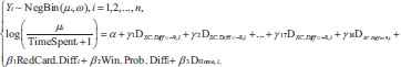
Fig. (1) illustrates the results of the stepwise variable selection procedure outlined in Section 2.3 for all considered leagues. These results take the form of direct multiplicative effects of the respective variables on the response variable (shots), where their linear coefficients are raised to the power of the exponent (e.g., eβˆ). A value of ”1.00” represents no effect, indicating that the respective variable was not selected for the final model. Values above (below) 1.00 correspond to positive (negative, respectively) multiplicative impacts on offensive output.
The score differential categories selected in the final model across nearly all leagues ranged from −4 to +4 (excluding 0, which serves as the baseline representing a tied game). Trailing teams tend to produce more shots (with their multiplication coefficients always > 1), while teams in the lead are less active (with coefficients < 1). Extreme score cases (e.g., differentials of ≥ 5 goals) are rarely selected, which can be attributed to smaller sample sizes and fewer minutes played in such scenarios, as well as the increased likelihood of non-trivial game dynamics that lead to such lopsided outcomes.
As for the other predictors potentially affecting playing style, these were selected in the final model across all five leagues. Weighted win probability consistently showed a strong positive association with a team’s offensive production, home teams tended to be slightly more active offensively, and red card differential had a significant negative impact on offensive output. The latter confirms the intuition that teams with more red cards (and thus fewer players on the field) are forced to play more defensively. The results for corners as an offensive output were similar to those for shots (see the supplement). For all the aforementioned effects, it is important to note that the other predictors included in our model are held constant, addressing potential confound-ing issues.
After stepwise selection identified the scoring differentials from −4 through +4 for adjustment of shots, we pursued the ad-hoc approach outlined in Section 2.3. We merged the extreme score differentials into their respective categories, starting with the largest absolute differential selected (4), creating the categories ”-4 or worse” and ”+4 or better”, and working our way down.
Rating the categories ”-2 or worse” and ”+2 or better” resulted in the model with the best BIC value, outperforming all previously considered models across all five leagues. This same model also performed best for corners as the offensive statistic. Based on these results, we adopted this model as the final one.
Stepwise variable selection results for 15 seasons (2008-2023) across five major European soccer leagues, converted into multiplicative effects of the respective variables on shots attempted. A value of ”1.00” indicates no effect (i.e., the variable was not selected), while coefficients above and below 1.00 represent positive and negative effects on shots, respectively. The score differential of 0 was not an explicit variable in the selection process (it served as the baseline) and is included here solely to represent the tied game scenario.
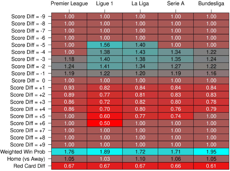
Fig. (2) illustrates the multiplicative effects of various scoring and red card differential categories on shot attempts (top) and corner kicks (bottom). Both predictors show a decrease in offensive output as the differential increases from negative to positive values, which aligns with the intuition and results are presented in Fig. (1). Red card differential has a noticeably stronger impact in magnitude compared to score differential. These findings are consistent across all five major European soccer leagues considered in this study.
3.2. Statistical Adjustment
Table 1 illustrates the largest positive and negative adjustments to shot production in each of the five European soccer leagues considered, along with the contextual breakdown of the game situations during which the shots were accumulated.
From the five largest positive adjustments, it is clear that the majority of shots were accumulated when the respective team was down by at least one player and mostly when they were ahead by at least one goal (both situations are typically less conducive to shot production, hence benefit-ing from the adjustment). The largest increase occurred for West Bromwich (”W Brom”) in the English Premier League, where the shot count rose from 14 to 30.1 after the adjustment. In addition to receiving a red card in the 11th minute, West Bromwich received a second red card in the 29th minute, leaving them to play 9 versus 11 for over 60 minutes. During this period, they accumulated 13 of their 14 shots. This factor outweighed their being behind in score for most of the game (which would typically encourage more shot production), resulting in the largest positive adjustment overall.
Multiplicative effects of scoring (left) and red card (right) differentials in the final selected model, fitted to 15 seasons (2008-2023) across five major European soccer leagues. The y-axis represents the coefficient by which a statistic (shot attempt or corner kick) accumulated during a game context, as dictated by the values on the x-axes (e.g., a score differential of +1 or a red card differential of -1), must be multiplied. When the game is tied and played at even strength, no adjustment is applied (multiplicative coefficient of 1).
Regarding the five largest negative adjustments (last five rows), the majority of shots by these teams were attempted when they were ahead by at least one player and at least one goal (situations that typically result in higher shot production hence, the adjustment reduces those numbers). The largest decrease occurred for Bordeaux in French Ligue 1, where their 31 actual shots were projected down to 11.2. They were down by two goals by the 17th minute and their opponent received red cards in the 39th and 45th minutes. Curiously, Bordeaux did not attempt a single one of their 31 shots until they were playing with a two-man advantage (11 vs 9), which, combined with being down 0-2 in the score, led to such a significant contextual adjustment.
Moreover, it is worth noting that both entries from the English Premier League in Table 1 came from the same game when Blackpool hosted West Bromwich Albion during 2010/11 season. Although Blackpool won the game 2-1, their 26 shot attempts against West Bromwich’s 14 do not account for the fact that the latter played with a two-man disadvantage (9 versus 11) for the majority of the game. The adjusted values, which project Blackpool down to 11.9 shots and West Bromwich up to 30.1, provide a more contextualized view of the game, reflecting West Bromwich’s admirable effort while playing 60+ minutes with 2 men down.
Lastly, although the home factor was shown to have a smaller effect compared to score and red card differentials, it still contributed to away teams receiving extra credit and home teams being adjusted downward. This is evident from the fact that all five of the largest negative adjustments occurred for teams playing at home, while 3 out of the 5 teams with the largest positive adjustments played away.
| League | Team | Opponent | Season | Total Shots | Actual Shots (& Minutes Played) When | ||||
|---|---|---|---|---|---|---|---|---|---|
| Actual | Adjusted | Up 1+ goal |
Down 1+ goal |
Up 1+ men |
Down 1+ men |
||||
| ENG | W Brom | @ Blackpool | 2010/11 | 14 | 30.1 (⇑) | 0 (0) | 13∗(78) | 0 (0) | 13∗(80) |
| ESP | Real Madrid | @ Espanyol | 2010/11 | 18 | 33.4 (⇑) | 13 (66) | 0 (0) | 0 (0) | 18 (88) |
| FRA | Caen | @ Troyes | 2015/16 | 15 | 25.1 (⇑) | 13∗(76) | 0 (0) | 0 (0) | 9 (37) |
| GER | Bayern Mun | Stuttgart | 2020/21 | 15 | 24.5 (⇑) | 12∗(76) | 0 (0) | 0 (0) | 14∗(82) |
| ITA | AS Roma | Chievo V | 2009/10 | 17 | 28.3 (⇑) | 15 (89) | 0 (0) | 0 (0) | 13 (79) |
| ... | ... | ... | ... | ... | ... | ... | ... | ... | ... |
| ENG | Blackpool | W Brom | 2010/11 | 26 | 11.9 (⇓) | 25∗(78) | 0 (0) | 26∗(80) | 0 (0) |
| ESP | Getafe | Deportivo | 2009/10 | 22 | 10.8 (⇓) | 0 (0) | 22∗(77) | 19∗(64) | 0 (0) |
| FRA | Bordeaux | Montpellier | 2021/22 | 31 | 11.2 (⇓) | 0 (0) | 31∗(93) | 31∗(65) | 0 (0) |
| GER | Eintracht | Stuttgart | 2010/11 | 30 | 20.0 (⇓) | 0 (0) | 12∗(26) | 26 (77) | 0 (0) |
| ITA | AS Roma | Venezia | 2021/22 | 43 | 26.6 (⇓) | 0 (0) | 29 (79) | 38 (69) | 0 (0) |
An analogous table of the five largest positive and negative adjustments for corners is available in the supplement. The findings are similar in that teams accumulating most of their corner shots while up by at least one man and/or one goal are adjusted downward, and vice versa.
CONCLUSION
We modeled teams’ offensive production, such as shot attempts and corner kicks, as a function of various factors that influence the implementation of specific tactics. We found that the model providing the best balance between quality of fit and interpretability was a Negative Binomial regression that included linear predictors for red card differential, home factor, and weighted win probability, with score differentials categorized into the following groups: ”-2 or worse”, ”-1”,
”0”, ”+1”, and ”+2 or better”. Both score and red card differentials negatively impacted teams’ offensive production, with the red card differential having a notably larger effect. These findings confirm the well-known intuition that teams with leads and/or fewer players on the field tend to play more defensively. Leading teams typically adopt a defensive strategy to protect their lead and secure the valuable 3 points (compared to 1 point for a draw), while teams with at least one player down are essentially forced into a more defensive approach due to being outnumbered. Additionally, the home factor consistently showed a positive effect on offensive production, though of relatively low magnitude. Lastly, the weighted win probability exhibited a strong positive association with offensive production, supporting the intuition that better teams (with higher betting odds) outperform their opponents. Controlling for this factor allowed for a more precise estimation of the effects of the other factors we adjusted for—score differential, red cards, and home indicator.
These results were consistent across all five major European soccer leagues and both statistical categories considered (shot attempts and corner kicks).
When applying the statistical adjustment, we projected each team’s offensive performance in a selected statistical category onto a tied home game played at even strength. This resulted in upward adjustments for statistics accumulated during periods when a team was leading and/or down at least one player (to account for contexts that are less conducive to offensive output), and vice versa. As a result, the largest impacts were observed in games with prolonged periods of imbalanced play (e.g., 9 or 10 players versus 11) and/or when one team maintained a lead. The home factor also played a role, but not to the same extent as score and red card differentials.
Our performance evaluation approach offers an alternative perspective compared to conventional box score statistics. Unlike traditional game totals, our method takes into account the context under which various offensive outputs were accumulated, potentially providing a more accurate reflection of the relative level of play between the two teams. Through several game examples, we demonstrated how traditional statistics might either understate or overstate a team’s performance and how our statistical adjustment addresses this issue. For instance, in the case of West Bromwich Albion’s valiant effort against Blackpool while down two men, our approach gives greater weight to offensive outputs accumulated while shorthanded and/or leading in score.
Conversely, our methodology downplays statistics accumulated when trailing and/or having a numerical advantage—situations more conducive to offensive production. This was the case with Bordeaux’s 31 shots, which occurred while they had a two-man advantage and trailed by two goals. These examples illustrate how our statistical adjustment provides an alternative view that gives more recognition to teams outperforming expectations given the game context (e.g., West Bromwich Albion played most of the game while down two men), while reducing the value of statistics accumulated in situations most favorable for offensive production (e.g., Bordeaux playing with a two-man advantage and trailing).
One avenue for future work would be to account for the exact minute in the game when an event (such as a shot or corner) occurred, rather than simply accumulating the total over a time period. This could provide insights into offensive tendencies as the game progresses, especially as the sense of urgency increases toward the end. Additionally, although we mentioned a World Cup elimination game as an illustration, it is important to note that this study focused on national club leagues, where there are no elimination games, and outcomes are assigned clear point values (3 points for a win, 1 point for a draw, and 0 points for a loss). A promising extension would be to explore the dynamics of competitions that place more emphasis on score differential—rather than points—to determine who advances to the next round. Examples include the Football Association Challenge Cup (FA Cup), the World Cup, and the Champions League elimination stages.
AUTHORS’ CONTRIBUTION
It is hereby acknowledged that all authors have accepted responsibility for the manuscript's content and consented to its submission. They have meticulously reviewed all results and unanimously approved the final version of the manuscript.
AVAILABILITY OF DATA AND MATERIALS
The authors confirm that the data supporting the findings of this research are available within the article.
ACKNOWLEDGEMENTS
The authors are grateful to the host institution for providing summer research funding.